Trading as a Probabilistic ProcessTrading as a Probabilistic Process
As mentioned in the previous post , involvement in the market occurs for a wide range of reasons, which creates structural disorder. As a result, trading must be approached with the understanding that outcomes are variable. While a setup may reach a predefined target, it may also result in partial continuation, overextension, no follow-through, or immediate reversal. We trade based on known variables and informed expectations, but the outcome may still fall outside them.
Therefore each individual trade should be viewed as a random outcome. A valid setup could lose; an invalid one could win. It is possible to follow every rule and still take a loss. It is equally possible to break all rules and still see profits. These inconsistencies can cluster into streaks, several wins or losses in a row, without indicating anything about the applied system.
To navigate this, traders should think in terms of sample size. A single trade provides limited insight, relevant information only emerges over a sequence of outcomes. Probabilistic trading means acting on repeatable conditions that show positive expectancy over time, while accepting that the result of any individual trade is unknowable.
Expected Value
Expected value is a formula to measure the long-term performance of a trading system. It represents the average outcome per trade over time, factoring in both wins and losses:
Expected Value = (Win Rate × Average Win) – (Loss Rate × Average Loss)
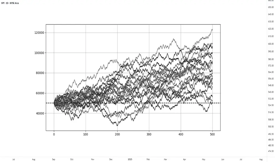
This principle can be demonstrated through simulation. A basic system with a 50% win rate and a 1.1 to 1 reward-to-risk ratio was tested over 500 trades across 20 independent runs. Each run began with a $50,000 account and applied a fixed risk of $1000 per trade. The setup, rules, and parameters remained identical throughout; the only difference was the random sequence in which wins and losses occurred.
While most runs clustered around a profitable outcome consistent with the positive expected value, several outliers demonstrated the impact of sequencing. When 250 trades had been done, one account was up more than 60% while another was down nearly 40%. In one run, the account more than doubled by the end of the 500 trades. In another, it failed to generate any meaningful profit across the entire sequence. These differences occurred not because of flaws in the system, but because of randomness in the order of outcomes.
These are known as Monte Carlo simulations, a method used to estimate possible outcomes of a system by repeatedly running it through randomized sequences. The technique is applied in many fields to model uncertainty and variation. In trading, it can be used to observe how a strategy performs across different sequences of wins and losses, helping to understand the range of outcomes that may result from probability.
Trading System Variations
Two different strategies can produce the same expected value, even if they operate on different terms. This is not a theoretical point, but a practical one that influences what kind of outcomes can be expected.
For example, System A operates with a high win rate and a lower reward-to-risk ratio. It wins 70% of the time with a 0.5 R, while System B takes the opposite approach and wins 30% of the time with a 2.5 R. If the applied risk is $1,000, the following results appear:
System A = (0.70 × 500) − (0.30 × 1,000) = 350 − 300 = $50
System B = (0.30 × 2,500) − (0.70 × 1,000) = 750 − 700 = $50
Both systems average a profit of $50 per trade, yet they are very different to trade and experience. Both are valid approaches if applied consistently. What matters is not the math alone, but whether the method can be executed consistently across the full range of outcomes.
Let’s look a bit closer into the simulations and practical implications.
The simulation above shows the higher winrate, lower reward system with an initial $100,000 balance, which made 50 independent runs of 1000 trades each. It produced an average final balance of $134,225. In terms of variance, the lowest final balance reached $99,500 while the best performer $164,000. Drawdowns remained modest, with an average of 7.67%, and only 5% of the runs ended below the initial $100,000 balance. This approach delivers more frequent rewards and a smoother equity curve, but requires strict control in terms of loss size.
The simulation above shows the lower winrate, higher reward system with an initial $100,000 balance, which made 50 independent runs of 1000 trades each. It produced an average final balance of $132,175. The variance was wider, where some run ended near $86,500 and another moved past $175,000. The drawdowns were deeper and more volatile, with an average of 21%, with the worst at 45%. This approach encounters more frequent losses but has infrequent winners that provide the performance required. This approach requires patience and mental resilience to handle frequent losses.
Practical Implications and Risk
While these simulations are static and simplified compared to real-world trading, the principle remains applicable. These results reinforce the idea that trading outcomes must be viewed probabilistically. A reasonable system can produce a wide range of results in the short term. Without sufficient sample size and risk control, even a valid approach may fail to perform. The purpose is not to predict the outcome of one trade, but to manage risk in a way that allows the account to endure variance and let statistical edge develop over time.
This randomness cannot be eliminated, but the impact can be controlled from position sizing. In case the size is too large, even a profitable system can be wiped out during an unfavorable sequence. This consideration is critical to survive long enough for the edge to express itself.
This is also the reason to remain detached from individual trades. When a trade is invalidated or risk has been exceeded, it should be treated as complete. Each outcome is part of a larger sample. Performance can only be evaluated through cumulative data, not individual trades.
Simulation
Fractal Phenomenon Proves Simulation Hypothesis?The humanity is accelerating towards the times when virtual worlds will get so realistic that their inhabitants gain consciousness without realizing they exist in a simulation. The idea that we might be living in a simulation was widely introduced in 2003 by philosopher Nick Bostrom. He argued that if the civilization can create realistic simulations, the probability that we are living in one is extremely high.
Modern games only render areas that the player is observing, much like how reality might function in a simulation. Similarly, texture of game environments update as soon as they are viewed, reinforcing the idea that observation determines what is rendered.
QUANTUM MECHANICS: The Ultimate Clue
Quantum Mechanics challenges our fundamental understanding of reality, revealing a universe that behaves more like a computational process than a physical construct. The wave function (Ψ) describes a probability distribution, defining where a particle might be found. However, upon measurement, the particle’s position collapses into a definite state, raising a paradox: why does the smooth evolution of the wave function lead to discrete outcomes? This behavior mirrors how digital simulations optimize resources by rendering only what is observed, suggesting that reality itself may function as an information-processing system.
The Born Rule reinforces this perspective by asserting that the probability of finding a particle at a given location is determined by the square of the wave function’s amplitude (|Ψ|²). This principle introduced probability into the very foundations of physics, replacing classical determinism with a probabilistic framework. Einstein famously resisted this notion, declaring, “God does not play dice,” yet Quantum Mechanics has since revealed that randomness and structure are not opposing forces but intertwined aspects of reality. If probability governs the fabric of our universe, it aligns with how simulations generate dynamic outcomes based on algorithmic rules rather than fixed physical laws.
One of the most striking paradoxes supporting the Simulation Hypothesis is Schrödinger’s Cat, which illustrates the conflict between quantum superposition and observation. In a sealed box, a cat is both alive and dead until an observer opens the box, collapsing the wave function into a single state. This suggests that reality does not exist in a definite form until it is observed—just as digital environments in a simulation are rendered only when needed.
Similarly, superposition demonstrates that a particle exists in multiple states until measured, while entanglement reveals that two particles can be instantaneously correlated across vast distances, defying classical locality. These phenomena hint at an underlying informational structure, much like a networked computational system where data is processed and linked instantaneously.
Hugh Everett’s Many-Worlds Interpretation (MWI) takes this concept further by suggesting that reality does not collapse into a single outcome but instead branches into parallel universes, where each possible event occurs. Rather than a singular, objective reality, MWI posits that we exist within a constantly expanding system of computational possibilities—much like a simulation running countless parallel computations. Sean Carroll supports this view, arguing that the wave function itself is the fundamental reality, and measurements merely reveal different branches of an underlying universal structure.
If our reality behaves like a quantum computational system—where probability governs outcomes, observation dictates existence, and parallel computations generate multiple possibilities—then the Simulation Hypothesis becomes a compelling explanation. The universe’s adherence to mathematical laws, discrete quantum states, and non-local interactions mirrors the behavior of an advanced simulation, where data is processed and rendered in real-time based on observational inputs. In this view, consciousness itself may act as the observer that dictates what is “rendered,” reinforcing the idea that we exist not in an independent, physical universe, but within a sophisticated computational framework indistinguishable from reality.
Fractals - Another Blueprint of the MATRIX?
Price movements wired by multi-cycles shaping market complexity. Long-term cycles define the broader trend, while short-term fluctuations create oscillations within that structure. Bitcoin’s movement influencing Altcoins exemplifies market entanglement—assets affecting each other, much like quantum particles. A single event in a correlated market can ripple across the entire system like in Butterfly effect. Just as a quantum particle exists in multiple states until observed, price action is a probability field—potential breakouts and breakdowns coexist until liquidity shifts. Before a definite major move, the market, like Schrödinger’s cat, remains both bullish and bearish until revealed by Fractal Hierarchy.
(Model using Weierstrass Function )
A full fractal cycle consists of multiple oscillations that repeat in a structured yet complex manner. These cycles reflect the inherent scale-invariance of market movements—where the same structural patterns appear.. By visualizing the full fractal cycle:
• We observe the relationship between micro-movements and macro-structures.
• We track the transformation of price behavior as the fractal unfolds across time.
• We avoid misleading interpretations that come from looking at an incomplete cycle, which may appear random or noisy
From Wave of Probability to Reality
1. Fractal Probability Waves – The market does not move in a straight line but rather follows a probabilistic fractal wave, where past structures influence future movements.
2. Emerging Reality – As the price action unfolds, these probability waves materialize, turning potential fractal paths into actual price trends.
3. Scaling Effect – The same cyclical behavior repeats at different scales (6H vs. 1W in this case), reinforcing the concept that price movements are self-similar and probabilistically driven.
If psychology of masses that shapes price dynamics is governed by mathematical sequences found in nature, it strongly supports the Simulation Hypothesis
Do you think we live in a simulation? Let’s discuss in comments!

$BTC1! Fib Simulation of Fractal (UPD)Perceiving the price action as a function of trading time justifies the quantitative approach in drawing geometric relationship between phases of cycles. Hence, it's safe for me to assume that market is a time fractal which has its own path regardless the collective opinions of the market participants. Logistic curve that reflects well the speed of information spreading made me ignore the voices of masses. The principle aligns with EMH - that the condition of the market is already reflected in the current price.
Impulsive and corrective waves are governed by golden rule in one way or the other. That's why I used fibonacci channels to build predictive models which reflect the interconnectedness of composite fractals to the whole cycle. By measuring the extreme levels of historic wave, the derived fibonacci channels exposed the timing, size and probability levels of the next ones.
In regular TA, people are wrongfully focused on covering their immediate expectations from the market, analyzing a narrow data range of the chart. Whereas, Fractal Analysis graphically shows how current price is interconnected with the entire history of fluctuations in a single probabilistic map.
In this update I fused earlier discovered structures and boundaries to the chart
Added more series of fib ratios derived from white triangle (src 0;1)
Linear boundaries of macro-fractal:
Implementation of fibs with big time Intervals:
As violet Fibs:
Other observations:
We're in a big triangle derived by linear extension 2021 tops and Full cycle (COVID - 2022 LOWS)
Source:
Implementation:
(On interactive chart it darkens till intersection)

$BTC: Fib Interference PatternAdded 2 other fib ratios for extending awareness about the presence of extra golden proportions.
Those are 0.146 and 0.887
2021 double tops define an important angle which is relevant to the chart in terms of its distinctive angle of the shift towards the side.
Given angle we could define the width of fibonacci channel by applying the Nov 2022 bottom:
Tops 2017 & 2021 applied to Coving bottom:
Establishing fabric of PriceTime based on its historic incline.
To increase further the awareness on waves of probability limits, the process can be repeated.
Tops 2013 & 2017 applied to 2011 Low
High angle fib channel related to timing:
2011 & 2013 Tops applied to August 2015 Low

TradingView Masterclass: Paper TradingIn this Masterclass, you’ll learn how to use our official paper trading tool. Paper trading gives trades the capability to test their trading skills in a simulated environment without risking real money. For all the new traders out there, you’ll want to make paper trading your best friend. Why? Have all the fun you want, practice endlessly, and never lose a dime.
Reminder: With Black Friday nearing (seriously… it’s coming soon), now is the time to master one of our most important tools. You’ll be ready to go the second you activate your upgraded account.
To get started, follow the steps below:
Step 1 - Click the ‘Trading Panel’ button located at the bottom of the chart.
Step 2 - Once you click the ‘Trading Panel’ button, a list of brokers in your region will appear, but also, at the very top, a Paper Trading account powered by yours truly, TradingView.
Step 3 - Click Paper Trading and you’ll now start the process of opening your free, simulated trading environment, entirely powered by us.
You made it! Time to celebrate! 🕺💃
Alright, let’s go a little deeper and talk about the buttons you’ll want to understand now that you’ve got your Paper Trading account opened.
While still having the Trading Panel open, click the button that says “Trade” and an order slip will appear. It’ll look like this:
As you get started, here are some tips to keep in mind:
Take Paper Trading seriously. Work Paper Trading as if it were a real account:
Record your trades, the reasons, the results obtained and the lessons learned.
Explore different approaches like intraday trading or swing trading.
Maintain emotional discipline, your trading strategy and risk management.
Practice, practice, practice - that’s what this is all about, getting better at trading through practice.
It gets better, because there are multiple ways to trade and customize your paper trading experience. Open the chart settings menu or right click on the chart, and you can add specific trading features to the chart as needed.
In-fact, we’ll explain all of the features available to you in the chart settings.
🟥🟦 Buy/Sell buttons :
When these are turned on, you’ll see a Buy and Sell button at the top right of the chart. When it comes to buying and selling, there are three primary order types:
Market (executed at the current market price),
Limit (executed at a defined specific value), and
Stop (executed when the price falls below a certain level).
👆 Instant Orders placement :
This option allows you to open positions at the market price by simply clicking the buy and sell buttons. You can choose the quantity by clicking on the number below the spread.
⏰ Play Sound for executions :
You can enable this option to receive an audible notification when a trade is executed, with eight different tones to choose from.
📲 Notifications :
Receive notifications for All events or Rejection orders only.
Tip : You can open the order panel by using the Shift + T shortcut or by right-clicking on a chart, then selectings Trade > Create a new order.
👁🗨 Positions :
Uncheck this box if you don’t want to see your active trading positions.
🔺🔻 Profit & loss :
This option allows you to view the profit and loss changes in your trades, which can displayed in both ticks and percentages.
🔃 Reverse button :
When enabled, a button is added to your active trading positions that allows you to reverse your trade.
👁 Orders :
See your current open unexecuted orders by checking this box.
🔺🔻👁 Brackets profit & loss :
It functions similarly to the Profit & Loss option, but for pending orders.
⏪ Executions :
It displays the past executed orders on the chart.
Execution labels :
Enable this option to view specific information about past execution orders, including trade direction, quantity, and executed price.
Extended price line for positions & orders :
It creates an extended horizontal line for your active trades.
⬅⬆➡ Orders & positions alignment :
You can move the alignment of your orders to Left, Center and Right in your charts.
🖥 Orders, Executions and Positions on screenshots :
Check this box if you want to download screenshots (shortcut: Ctrl + Alt + S) with active and pending orders.
Thanks for reading and we hope this tutorial helps you get started! We look forward to reading your feedback.
- TradingView Team

XU100 and others (relatively cheap)From P/E perspective: cheap assets and baskets (markets) are on target. We can expect bollinger band as reference to movements (a kind of threshold). Positive deviations from upper band may be expected

ANSS AnSys The Software Simulation Engine For Everything AI Ansys, Inc. is an American company based in Canonsburg, Pennsylvania. It develops and markets CAE/multiphysics engineering simulation software for product design, testing and operation and offers its products and services to customers worldwide.
Opening positions under $220 and attempting to hold for $300

S&P 500 ETF MicroFractal I 15mSource of General Fractal of current decline rhymed to historic pattern:
Breaking below shallow upward angle switch to:
Doesn't hold 394.83? Switch to chart below if you believe that market should make a recession type of decline:
If you still feel optimistic about the economy and your analysis doesn't reflect apocalyptic drops:

What if this time isn't different? A 2 year scenario projecting the financial crisis of 2008-2009 into the future
Chart (W, LOG):
Stocks: The averaged futures for SPX, NAS and DJ were weighted so that a 1 point change will imply the same change in $ terms. (For weights see www.barchart.com
200MA, 50MA, and 21MA
Today's price and date: at the intersection of the cross.
Financial crisis: Purple box on the left
Implied scenario: Purple box on the right. Left edge starts 10/5/2022 ("Today" .. for the next 10 min)
Methodology:
The scenario is a scaled up copy of the box at 2008-2009. It is stretched to fit the current price, and it's 3 MA's.
For simplicity the price / time aspect ratio was preserved.
Criteria for 'best fit' (using IEI ) were the absolute level and curvature of the 3 MA's. In other words, the distance between the MA's, their slopes, and the speed each slope was changing.
Main Implications:
The scenario implies a crash (ripped from Feb 2009) beyond the March, 2020 COVID low, as far as the highs of 2015. This is after the end of QE, when Greece went into default and the Yen was devalued overnight .
"Bottom" of the implied crash is one year from today (10/5/2022).
Notes:
1. IEI : I eyeballed it
2. Gann would not be happy and the result could be different on a RENKO or equivalent treatment of time (a great follow up idea)
3. The night the Yen was devalued I held positions in gold in bond futures (GC and ZB). I have used stops without exceptions from that day on.
best graphics:

Ethereum Simulation - NeutralHope the momentum does not break and keeps heading higher and higher.
Please share your thoughts, ideas, and evaluation. If you liked this analysis, smash the like button which will motivate me to publish more of my analysis often. Thanks for viewing!
Disclaimer: There is a very high degree of risk involved in trading. This is my very personal analysis and it does not intend to be a bit of advice in anyways.

Bitcoin SimulationSimulation worth a million words. Your likes and comments are highly appreciated. Good luck!

