THF Crossover and Trend Signals Golden & Death Cross with VolumeScript Overview:
This Pine Script is designed to assist traders in identifying key buy/sell signals and major trend changes on the chart using Exponential Moving Averages (EMA) and Simple Moving Averages (SMA), as well as visualizing Golden Cross and Death Cross events. The script also includes a volume indicator to highlight the volume trading activity in relation to the price movements.
Key Features:
1. Moving Averages:
EMA 21: Exponential Moving Average over a 21-period, shown in green.
EMA 50: Exponential Moving Average over a 50-period, shown in yellow.
SMA 50: Simple Moving Average over a 50-period, shown in red.
SMA 200: Simple Moving Average over a 200-period, shown in blue.
2. Signals:
Buy Signal: Generated when EMA 21 crosses above SMA 50, indicating a potential upward trend. Displayed with a green label below the price bar.
Sell Signal: Generated when EMA 21 crosses below SMA 50, indicating a potential downward trend. Displayed with a red label above the price bar.
3. Golden Cross (Bullish Trend):
A Golden Cross occurs when EMA 50 crosses above SMA 200, which often signals the start of a long-term upward trend. The signal is displayed with a yellow label below the price bar.
4. Death Cross (Bearish Trend):
A Death Cross occurs when EMA 50 crosses below SMA 200, which often signals the start of a long-term downward trend. The signal is displayed with a blue label above the price bar.
5. Volume Indicator:
The volume is plotted as colored columns. Green indicates higher volume than the 20-period moving average, and red indicates lower volume.
A Volume Moving Average (SMA 20) is also plotted to compare volume changes over time.
How the Script Works:
1. The EMA and SMA lines are plotted on the chart, providing a visual representation of the short- and long-term trends.
2. Buy/Sell signals are triggered based on the crossover between EMA 21 and SMA 50, helping to identify potential entry and exit points.
3. The Golden Cross and Death Cross indicators highlight major trend reversals based on the crossover between EMA 50 and SMA 200, providing clear visual cues for long-term trend changes.
4. Volume is displayed alongside price movements, offering insight into the strength or weakness of a trend.
Key Customizations:
Moving Average Periods: Users can modify the lengths of the EMAs and SMAs for customized analysis.
Volume Moving Average Period: The script allows for adjustment of the volume moving average period to suit different market conditions.
Signal Visibility: The size and color of the buy, sell, Golden Cross, and Death Cross signals can be easily customized to make them more prominent on the chart.
Conclusion:
This script is ideal for traders looking to combine price action with volume analysis, using key technical indicators such as EMA, SMA, Golden Cross, and Death Cross to make informed decisions in trending markets.
---
This explanation covers all aspects of the script and provides a clear understanding of its functionality, which is helpful for sharing the script or using it as an educational resource.
Breadth Indicators

OBV Oscillator with Divergence CirclesCredit to original code from the 'PPO Divergence alerts' by Scarf and OBV Oscillator by LazyBear is used as the input.
Replication of Lunndi 'OBV Divergence Alerts (BETA)' script with additional divergence logic implemented.
OBV-based divergence logic adapted from RSI divergence logic added in addition to existing divergence logic.
Modify length and smoothing to suit your trading style. Open source free for use.

Alprof Strategyyou can get strategy by TS this strategy you can get a entry point
you can get strategy by TS this strategy you can get a entry point
you can get strategy by TS this strategy you can get a entry point
you can get strategy by TS this strategy you can get a entry point
you can get strategy by TS this strategy you can get a entry point
you can get strategy by TS this strategy you can get a entry point

High Volume Buyers/Sellers+High Volume Buyers/Sellers+
This indicator helps traders spot bars where unusually high or extreme volume occurs, indicating strong buying or selling pressure.
How it works:
Calculates a volume moving average (SMA) over a user-defined period.
Marks bars where the current volume exceeds:
High Volume Multiplier → small green circle (bullish) or red circle (bearish).
Extreme Volume Multiplier → small green up-triangle (bullish) or red down-triangle (bearish).
Settings:
Volume MA Period → Number of bars used to calculate the average volume.
High Volume Multiplier → Threshold to define high volume.
Extreme Volume Multiplier → Threshold to define extreme volume.
Show Extreme Volume Signals → Option to enable or disable extreme volume markers.
Usage tips:
Apply this indicator on a clean chart to visually highlight momentum bursts or exhaustion points.
It works well for both intraday and swing trading strategies where volume confirmation matters.
⚠ Note: This script only displays on-chart markers and does not plot any lines or indicators.

3 EMA trong 1 NTT CAPITALThe 3 EMA in 1 NTT CAPITAL indicator provides an overview of the market trend with three EMAs of different periods, helping to identify entry and exit points more accurately, thus supporting traders in making quick and effective decisions.

combo EMAS Session [Indexprofx]🧠 Description:
This indicator highlights the New York and London trading sessions directly on the chart, offering a clear visual reference for intraday trading.
It is a complementary tool designed to work seamlessly with our main system: Intraday Signal.
✔️ Displays the most active market hours.
✔️ Enhances precision in entry and exit decisions.
✔️ Perfect for XAUUSD (Gold) traders and other high-volatility instruments.
🧠 Description:
This indicator plots three key Exponential Moving Averages (EMAs) to help traders identify market trends and potential entry/exit points with precision:
EMA 8 (Green) – Fast trend, useful for scalping or short-term signals
EMA 50 (Blue) – Mid-term trend filter
EMA 150 (Red) – Long-term bias and trend direction
It is part of the IndexProFX toolkit and integrates smoothly with other tools like Intraday Signal and Session Zones for enhanced confluence trading.
✔️ Clean structure
✔️ Easy-to-read color-coded EMAs
✔️ Supports scalping, day trading, and swing trading strategies

3 EMAS Indexprofx🧠 Description:
This indicator plots three key Exponential Moving Averages (EMAs) to help traders identify market trends and potential entry/exit points with precision:
EMA 8 (Green) – Fast trend, useful for scalping or short-term signals
EMA 50 (Blue) – Mid-term trend filter
EMA 150 (Red) – Long-term bias and trend direction
It is part of the IndexProFX toolkit and integrates smoothly with other tools like Intraday Signal and Session Zones for enhanced confluence trading.
✔️ Clean structure
✔️ Easy-to-read color-coded EMAs
✔️ Supports scalping, day trading, and swing trading strategies

IB Breakout Strategy with Fib, CVD, and DivergenceEntry rules and signals- I wait for the 5min IB(initial balance) to form every session for eg-(first 5min candle of london session or ny session, marking top wick to bottom wick of first 5 min candle with a midpoint in that zone.Then look for CVD(cumulative volume delta) if it's alining with my analysis.I also mark previous session fib levels for scalp entries on .618 or .78 level.Also i do mark previous day VAH(value area high),VAL(value area low) and POC(point of control) for better understanding of direction.
Initial stop loss and take profit values-Initial stop loss varies from 200$ to 500$ and take profit varies from 250$ to 500$.
Number of contracts you plan to trade based on system stats and risk management-I plan to trade 1-2 contracts until i reach the safety net.Once safety net is achieved based on my entry level i decide the contract size which varies from 1-4 contracts.
Trade management and any trailing stop methods-I trail the stop once i feel like there's enough room for the trade.I manage the trade on the basis of strength of a candle, if its taking much time without strength i exit the trade.


Heikin Ashi Trend Strategy (Beginner)FOR BEGINNERS
Perfect! Below is a custom Pine Script for TradingView that:
Uses Heikin Ashi candles
Shows buy/sell signals based on trend conditions:
3+ green/red Heikin Ashi candles
Price above/below 20 EMA
RSI filter for momentum

Momentum & stoch rsimomentum and stochastic rsi indicator ideal for day trading. momenum is set to 80 for a smooth and safe analysis.

Oz SIGNAL PRO v6 is a powerful 15-minute trend-following indicator tailored for precision trading. It detects Break of Structure (BOS) and CHoCH signals with built-in volume confirmation and overlays premium/discount zones directly on the chart. The indicator includes:
🔹 Visual buy/sell labels at breakout points
🔸 Dynamic EMA and VWAP for trend filtering
🟩 Automatic support/resistance zones
🔔 Alert-ready for signal automation
Ideal for intraday traders seeking clean, high-confidence signals.
Upgrade-ready: Easily extend with FVGs, order blocks, liquidity sweeps & backtesting.

D15 Precision IndicatorD15 Precision Indicator
The D15 Precision Indicator is a high-accuracy intraday trading tool optimized for 15-minute charts. It identifies precise BUY and SELL signals only when all key conditions align:
✅ Price above/below EMA 21 & EMA 50
✅ Price above/below VWAP
✅ Price within predefined support/resistance zones
✅ Break of Structure (BOS) confirmed by pivot levels
✅ High-volume breakout candle
✅ Optional confirmation from previous candles for added precision
The script includes:
Clear visual arrows (BUY/SELL)
Dynamic background highlights for signals
Support/Resistance zone boxes
All key indicators plotted (EMA, VWAP, zones)
Ideal for disciplined traders aiming for 80%+ win rate through strict signal filtering and visual clarity.

STMD Indicator PROThe STMD Indicator PRO is designed for traders looking to capture strong trends using moving average alignment and the powerful Elephant Bar pattern, popularized by Oliver Velez.
📋 How it works?
✔ Simple Moving Averages:
SMA 8 (Black)
SMA 13 (Purple)
SMA 20 (Blue)
SMA 200 (Red, optional filter)
✔ Signal conditions:
All SMAs aligned and trending in the same direction
Price near the short-term SMAs
A strong candle (Elephant Bar) with a big body and small opposite wick
Signal only on the first or second consecutive candle of the same color
✅ Features
✔ Background color showing trend bias
✔ Alerts ready: STMD Buy and STMD Sell
✔ Optional SMA 200 filter for higher timeframe confirmation
📌 Disclaimer: This script is for educational purposes only. Not financial advice.

Bollinger Bottom + Middle Lines with Inline TextThis script visualizes key Bollinger Band levels based on two different SMAs (20 & 50 periods), with clear labeling and a smart price table.
🔸 Features:
Draws lower and middle Bollinger Band lines for both SMA(20) and SMA(50)
Inline text at the end of each line instead of default labels (cleaner view)
A dynamic table in the top-right corner, sorted from highest to lowest level
Color-coded rows:
▪️ Orange → BB20 Mid & BB20 Lower
▪️ Green → BB50 Mid & BB50 Lower
Auto-updates each bar without cluttering the chart
✅ Ideal for identifying technical accumulation zones
✅ Suitable for investors using scaling-in strategies or mean-reversion logic

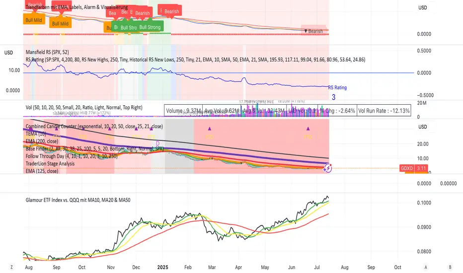
Glamour ETF Index vs. QQQ mit MA10, MA20 & MA50Stan Weinstein uses the term "Glamour Index" as a sentiment indicator to assess how speculative or overheated the stock market is. The Glamour Index measures the relationship between so-called "glamour stocks" (trendy stocks, hyped stocks with high media attention and sometimes extreme price increases) and solid, more conservative stocks. Weinstein uses this index to: 1) Analyze market sentiment – particularly whether the market is in a speculative euphoria phase.
2) Identify warning signs of a potential top formation or an impending downturn.
My basket compares performance against the QQQ (alternatively, SPY or any other benchmark is also possible).
My basket consists of the ETFs in the ARK universe, as well as other growth ETFs such as IPO, FFTY, and QQQJ.

RSI with Background Colorhis script implements a trading strategy based on an EMA (Exponential Moving Average) crossover, confirmed by the RSI (Relative Strength Index), and includes a built-in stop-loss and take-profit.

Turtle Trading System + ATR Trailing StopIndicator Description: Turtle ATR Trailing Stop
The **Turtle ATR Trailing Stop** is a technical indicator designed to enhance the classic Turtle Trading System by incorporating a dynamic trailing stop based on the Average True Range (ATR). This indicator is ideal for traders seeking to manage risk and lock in profits on both long and short positions in trending markets.
Key Features:
- Turtle Trading Levels: Calculates the 20-day highest high and lowest low to identify potential breakout points, a core principle of the Turtle Trading System.
- ATR-Based Trailing Stop: Utilizes a trailing stop that adjusts dynamically based on a multiple of the ATR (default multiplier: 2.0), providing a volatility-adjusted exit mechanism.
- Position Flexibility: Supports both long and short positions, with the trailing stop positioned below the highest price for long trades and above the lowest price for short trades.
- Smooth Updates: The trailing stop updates on each bar, ensuring a more responsive adjustment to price movements, rather than only on new highs or lows.
- Reset Mechanism: Automatically resets the trailing stop when the price deviates significantly (configurable threshold, default 0.1%), adapting to major trend reversals.
- Alerts: Includes customizable alerts that trigger when the price reaches the trailing stop level, notifying traders of potential exit points.
- Debugging Tools: Features an on-chart debug table displaying ATR, Close, Highest Price, Lowest Price, Potential Stop, and Trailing Stop values for real-time analysis.
How It Works:
- For **Long Positions**: The trailing stop starts below the initial close price (minus 2*ATR) and moves up as the highest price increases, locking in profits while trailing at a fixed ATR distance.
- For **Short Positions**: The trailing stop starts above the initial close price (plus 2*ATR) and moves down as the lowest price decreases, protecting against upward price movements.
- The stop resets if the price falls (for long) or rises (for short) beyond the set threshold, ensuring adaptability to new market conditions.
Customization:
- Period Settings: Adjust the length for highs/lows (default 20) and ATR period (default 14).
- ATR Multiplier: Modify the distance of the trailing stop (default 2.0).
- Reset Threshold: Fine-tune the percentage at which the stop resets (default 0.1%).
- Position Type: Switch between "Long" and "Short" modes via input settings.
Usage:
Apply this indicator to any chart in TradingView, set your preferred parameters, and monitor the trailing stop line (yellow) alongside the Turtle highs (red) and lows (blue). Use the debug table to validate calculations and set alerts to stay informed of stop triggers.
This indicator combines the trend-following strength of the Turtle System with a flexible, ATR-based stop-loss strategy, making it a powerful tool for both manual and automated trading strategies.

Intraday vs Overnight OBV🔍 Purpose
This indicator provides a volume-weighted cumulative flow model that mimics On-Balance Volume (OBV) logic but splits the volume impact into intraday vs. overnight sessions. It allows traders to track how volume contributes to price movement in each session and identify whether buying/selling pressure is stronger during or outside of regular trading hours.
This indicator attempts to alleviate some of the downfalls of the standard OBV indicator, which only looks at total volume and total direction. The price of stocks generally behaves extremely differently during market hours and outside market hours, and many of the large moves happen outside of regular market hours on low volume.
⚙️ Core Features
1) OBV-style calculation:
If price increases → volume is added to the OBV stream.
If price decreases → volume is subtracted.
If price is flat → OBV remains unchanged.
2) Session splitting:
Intraday session: movement from today's open to close.
Overnight session: movement from yesterday’s close to today’s open.
Volume is split proportionally between these two periods based on user input.
3) Four visualization modes:
"Intraday" — plots only OBV from intraday price movement.
"Overnight" — plots only OBV from overnight price movement.
"Aggregate" — plots the sum of intraday and overnight OBV for a holistic view.
"Both Intraday and Overnight" — plots intraday and overnight OBV separately on the same chart.
📐 Inputs
1) Synthetic OBV Type:
"Intraday" — Show OBV from open to close only.
"Overnight" — Show OBV from prior close to today's open only.
"Aggregate" — Show a single line combining both.
"Both Intraday and Overnight" — Show both lines on the same chart.
2) Estimated Overnight Volume %:
Percentage of total daily volume assumed to occur during extended hours.
The rest is allocated to regular session (intraday).
Default: 20% overnight, 80% intraday.
🧮 How It Works
Volume Splitting:
Total bar volume is split into overnight Volume and intraday Volume:
Intraday change is the difference between today’s close and open.
Overnight change is the difference between today’s open and yesterday’s close.
Session OBV Calculations:
OBV is incremented/decremented by the session's allocated volume, depending on whether the session’s price change was positive or negative.
Aggregate OBV:
Combines both session deltas for a holistic volume flow view.
📊 Interpretation
Rising OBV (any stream) suggests accumulation; falling OBV suggests distribution.
Divergences between price and OBV lines (especially overnight vs. intraday) can reveal where hidden buying/selling is occurring.
Comparing intraday vs overnight OBV can help:
Spot whether institutional demand is building off-hours.
Detect retail vs. institutional behavior (retail trades often dominate intraday; institutional may prefer after-hours).
💡 Use Cases
Identify whether overnight gaps are supported by overnight volume momentum.
Detect accumulation in low-volume overnight sessions.
Compare intraday and overnight strength during earnings season or news events.
Complement traditional OBV by seeing session-based breakdowns.

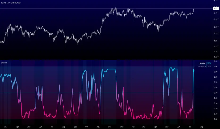
Crypto Breadth | AlphaNatt\ Crypto Breadth | AlphaNatt\
A dynamic, visually modern market breadth indicator designed to track the strength of the top 40 cryptocurrencies by measuring how many are trading above their respective 50-day moving averages. Built with precision, branding consistency, and UI enhancements for fast interpretation.
\ 📊 What This Script Does\
* Aggregates the performance of \ 40 major cryptocurrencies\ on Binance
* Calculates a \ breadth score (0.00–1.00)\ based on how many tokens are above their moving averages
* Smooths the breadth with optional averaging
* Displays the result as a \ dynamic, color-coded line\ with aesthetic glow and gradient fill
* Provides automatic \ background zones\ for extreme bullish/bearish conditions
* Includes \ alerts\ for key threshold crossovers
* Highlights current values in an \ information panel\
\ 🧠 How It Works\
* Pulls real-time `close` prices for 40 coins (e.g., XRP, BNB, SOL, DOGE, PEPE, RENDER, etc.)
* Compares each coin's price to its 50-day SMA (adjustable)
* Assigns a binary score:
• 1 if the coin is above its MA
• 0 if it’s below
* Aggregates all results and divides by 40 to produce a normalized \ breadth percentage\
\ 🎨 Visual Design Features\
* Smooth blue-to-pink \ color gradient\ matching the AlphaNatt brand
* Soft \ glow effects\ on the main line for enhanced legibility
* Beautiful \ multi-stop fill gradient\ with 16 transition zones
* Optional \ background shading\ when extreme sentiment is detected:
• Bullish zone if breadth > 80%
• Bearish zone if breadth < 20%
\ ⚙️ User Inputs\
* \ Moving Average Length\ – Number of periods to calculate each coin’s SMA
* \ Smoothing Length\ – Smooths the final breadth value
* \ Show Background Zones\ – Toggle extreme sentiment overlays
* \ Show Gradient Fill\ – Toggle the modern multicolor area fill
\ 🛠️ Utility Table (Top Right)\
* Displays live breadth percentage
* Shows how many coins (e.g., 27/40) are currently above their MA
\ 🔔 Alerts Included\
* \ Breadth crosses above 50%\ → Bullish signal
* \ Breadth crosses below 50%\ → Bearish signal
* \ Breadth > 80%\ → Strong bullish trend
* \ Breadth < 20%\ → Strong bearish trend
\ 📈 Best Used For\
* Gauging overall market strength or weakness
* Timing trend transitions in the crypto market
* Confirming trend-based strategies with broad market support
* Visual dashboard in macro dashboards or strategy overlays
\ ✅ Designed For\
* Swing traders
* Quantitative investors
* Market structure analysts
* Anyone seeking a macro view of crypto performance
Note: Not financial advise
Last xHL📈 Last xHL – Visualize Key Highs and Lows
This script highlights the most recent significant highs and lows over a user-defined period, helping traders quickly identify key support and resistance zones.
🔍 Features:
Highest High (HH) and Highest Close/Open (HC) lines
Lowest Low (LL) and Lowest Close/Open (LC) lines
Dynamic updates with each new bar
Gradient-filled zones between HH–HC and LL–LC for visual clarity
⚙️ Customization:
Adjustable lookback period (_length) to suit your trading style
Color-coded lines and fills for quick interpretation
🧠 Use Case:
This tool is ideal for traders who want to:
Spot potential breakout or reversal zones
Identify price compression or expansion areas
Enhance their technical analysis with visual cues
This script is for educational and informational purposes only. It does not constitute financial advice. Always do your own research before making trading decisions.

Candle Emotion Oscillator [CEO]Candle Emotion Oscillator (CEO) - Revolutionary User Guide
🧠 World's First Market Psychology Oscillator
The Candle Emotion Oscillator (CEO) is a groundbreaking indicator that measures market emotions through pure candle price action analysis. This is the first oscillator ever created that translates candle patterns into psychological states, giving you unprecedented insight into market sentiment.
🚀 Revolutionary Concept
What Makes CEO Unique
100% Pure Price Action: No volume, no external data - just candle analysis
Market Psychology: Measures actual emotions: Fear, Greed, Panic, Euphoria
Never Been Done Before: First oscillator to analyze market emotions
Exhaustion Prediction: Detects emotional fatigue before reversals
Fast Response: Perfect for your 2-5 minute scalping setup
The Four Core Emotions
🟢 GREED (Positive Values)
What it measures: Market conviction and decisiveness
Candle Pattern: Large bodies, small wicks
Psychology: Traders are confident and decisive
Oscillator: Positive values (0 to +100)
Trading Implication: Trend continuation likely
🔴 FEAR (Negative Values)
What it measures: Market uncertainty and indecision
Candle Pattern: Small bodies, large wicks
Psychology: Traders are uncertain and hesitant
Oscillator: Negative values (0 to -100)
Trading Implication: Consolidation or reversal likely
🚀 EUPHORIA (Extreme Positive)
What it measures: Excessive optimism and buying pressure
Candle Pattern: Large green bodies with upper wicks
Psychology: Extreme bullish sentiment
Oscillator: Values above +60
Trading Implication: Overbought, reversal warning
💥 PANIC (Extreme Negative)
What it measures: Capitulation and selling pressure
Candle Pattern: Large red bodies with lower wicks
Psychology: Extreme bearish sentiment
Oscillator: Values below -60
Trading Implication: Oversold, reversal opportunity
📊 Visual Elements Explained
Main Components
Thick Colored Line: Primary emotion oscillator
Green: Greed (positive emotions)
Red: Fear (negative emotions)
Bright Green: Euphoria (extreme positive)
Dark Red: Panic (extreme negative)
Thin Blue Line: Emotion trend (longer-term context)
Background Gradient: Emotional intensity
Darker = stronger emotions
Lighter = weaker emotions
Diamond Signals: 🔶 Emotional exhaustion detected
Rocket Signals: 🚀 Extreme euphoria warning
Explosion Signals: 💥 Extreme panic warning
Information Table (Top Right)
