Trend Range Detector (Zeiierman)█ Overview
Trend Range Detector (Zeiierman) is a market structure tool that identifies and tracks periods of price compression by forming adaptive range boxes based on volatility and price movement. When prices remain stable within a defined band, the script dynamically draws a range box; when prices break out of that structure, the box highlights the breakout in real-time.
By combining a volatility-based envelope with a custom weighted centerline, this tool filters out noise and isolates truly stable zones — providing a clean framework for traders who focus on accumulation, distribution, breakout anticipation, and reversion opportunities.
Whether you're range trading, spotting trend consolidations, or looking for volatility contractions before major moves, the Trend Range Detector gives you a mathematically adaptive, visually intuitive structure that maps the heartbeat of the market.
█ How It Works
⚪ Range Formation Engine
The core of this indicator revolves around two conditions:
Distance Filter: The maximum distance between all recent closes and a dynamic centerline must remain within a volatility envelope.
Volatility Envelope: Based on an ATR(2000) multiplied by a user-defined factor to account for broader market volatility trends.
If both conditions are satisfied over the most recent length bars, a range box is drawn to visually anchor the zone.
⚪ Dynamic Breakout Coloring
When price breaks out of the top or bottom of the active range box, the box color shifts in real-time:
Blue Boxes represent areas where price has remained within a defined volatility envelope over a sustained number of bars. These zones reflect stable, low-volatility periods, often associated with consolidation, equilibrium, or market indecision.
Green Boxes for bullish breakouts.
Red Boxes for bearish breakdowns.
This allows traders to visually spot transitions from consolidation to expansion phases without relying on lagging signals.
█ Why Use a Weighted Close Instead of SMA?
A standard Simple Moving Average (SMA) treats all past closes equally, which works well in theory, but not in dynamic, fast-shifting markets. In this script, we replace the traditional SMA with a speed-weighted average that reflects how aggressively the market has moved bar-to-bar.
⚪ Here's why it matters:
Bars with higher momentum (larger price differences between closes) are given more weight.
Slow, sideways candles (typical in noise or low volume) contribute less to the calculated centerline.
This method creates a more accurate snapshot of market behavior, especially during volatile phases. As a result, the indicator adapts to market conditions more effectively, helping traders identify real consolidation zones, not just average lines distorted by flat bars or noise.
█ How to Use
⚪ Range Detection
Boxes form only when price remains consistently close to the speed-weighted mean.
Helps identify sideways zones, consolidations, and low-volatility structures where price is “charging up.”
⚪ Breakout Confirmation
Once price exits the top or bottom boundary, the box immediately highlights the direction of the break.
Use this signal in conjunction with your own momentum, volume, or trend filters for higher-confidence trades.
█ Settings
Minimum Range Length: Number of candles required for a valid range to form.
Range Width Multiplier: Adjusts the envelope around the weighted average using ATR(2000).
Highlight Box Breaks: Enables real-time coloring of breakouts and breakdowns for immediate visual feedback.
-----------------
Disclaimer
The content provided in my scripts, indicators, ideas, algorithms, and systems is for educational and informational purposes only. It does not constitute financial advice, investment recommendations, or a solicitation to buy or sell any financial instruments. I will not accept liability for any loss or damage, including without limitation any loss of profit, which may arise directly or indirectly from the use of or reliance on such information.
All investments involve risk, and the past performance of a security, industry, sector, market, financial product, trading strategy, backtest, or individual's trading does not guarantee future results or returns. Investors are fully responsible for any investment decisions they make. Such decisions should be based solely on an evaluation of their financial circumstances, investment objectives, risk tolerance, and liquidity needs.
Indicators and strategies

BE-Indicator Aggregator toolkit█ Overview:
BE-Indicator Aggregator toolkit is a toolkit which is built for those we rely on taking multi-confirmation from different indicators available with the traders. This Toolkit aid's traders in understanding their custom logic for their trade setups and provides the summarized results on how it performed over the past.
█ How It Works:
Load the external indicator plots in the indicator input setting
Provide your custom logic for the trade setup
Set your expected SL & TP values
█ Legends, Definitions & Logic Building Rules:
Building the logic for your trade setup plays a pivotal role in the toolkit, it shall be broken into parts and toolkit aims to understand each of the logical parts of your setup and interpret the outcome as trade accuracy.
Toolkit broadly aims to understand 4 types of inputs in "Condition Builder"
Comments : Line which starts with single quotation ( ' ) shall be ignored by toolkit while understanding the logic.
Note: Blank line space or less than 3 characters are treated equally to comments.
Long Condition: Line which starts with " L- " shall be considered for identifying Long setups.
Short Condition: Line which starts with " S- " shall be considered for identifying Short setups.
Variables: Line which starts with " VAR- " shall be considered as variables. Variables can be one such criteria for Long or short condition.
Building Rules: Define all variables first then specify the condition. The usual declare and assign concept of programming. :p)
Criteria Rules: Criteria are individual logic for your one parent condition. multiple criteria can be present in one condition. Each parameter should be delimited with ' | ' key and each criteria should be delimited with ' , ' (Comma with a space - IMPORTANT!!!)
█ Sample Codes for Conditional Builder:
For Trading Long when Open = Low
For Trading Short when Open = High with a Red candle
'Long Setup <---- Comment
L-O|E|L
' E <- in the above line refers to Equals ' = '
'Short Setup
S-AND:O|E|H, O|G|C
' 2 Criteria for used building one condition. Since, both have to satisfied used "AND:" logic.
Understanding of Operator Legends:
"E" => Refers to Equals
"NE" => Refers to Not Equals
"NEOR" => Logical value is Either Comparing value 1 or Comparing value 2
"NEAND" => Logical value is Comparing value 1 And Comparing value 2
"G" => Logical value Greater than Comparing value 1
"GE" => Logical value Greater than and equal to Comparing value 1
"L" => Logical value Lesser than Comparing value 1
"LE" => Logical value Lesser than and equal to Comparing value 1
"B" => Logical value is Between Comparing value 1 & Comparing value 2
"BE" => Logical value is Between or Equal to Comparing value 1 & Comparing value 2
"OSE" => Logical value is Outside of Comparing value 1 & Comparing value 2
"OSI" => Logical value is Outside or Equal to Comparing value 1 & Comparing value 2
"ERR" => Logical value is 'na'
"NERR" => Logical value is not 'na'
"CO" => Logical value Crossed Over Comparing value 1
"CU" => Logical value Crossed Under Comparing value 1
Understanding of Condition Legends:
AND: -> All criteria's to be satisfied for the condition to be True.
NAND: -> Output of AND condition shall be Inversed for the condition to be True.
OR: -> One of criteria to be satisfied for the condition to be True.
NOR: -> Output of OR condition shall be Inversed for the condition to be True.
ATLEAST:X: -> At-least X no of criteria to be satisfied for the condition to be True.
Note: "X" can be any number
NATLEAST:X: -> Output of ATLEAST condition shall be Inversed for the condition to be True
WASTRUE:X: -> Single criteria WAS TRUE within X bar in past for the condition to be True.
Note: "X" can be any number.
ISTRUE:X: -> Single criteria is TRUE since X bar in past for the condition to be True.
Note: "X" can be any number.
Understanding of Variable Legends:
While Condition Supports 8 Types, Variable supports only 6 Types listed below
AND: -> All criteria's to be satisfied for the Variable to be True.
NAND: -> Output of AND condition shall be Inversed for the Variable to be True.
OR: -> One of criteria to be satisfied for the Variable to be True.
NOR: -> Output of OR condition shall be Inversed for the Variable to be True.
ATLEAST:X: -> At-least X no of criteria to be satisfied for the Variable to be True.
Note: "X" can be any number
NATLEAST:X: -> Output of ATLEAST condition shall be Inversed for the Variable to be True
█ Sample Outputs with Logics:
1. RSI Indicator + Technical Indicator: StopLoss: 2.25 against Reward ratio of 1.75 (3.94 value)
Plots Used in Indicator Settings:
Source 1:- RSI
Source 2:- RSI Based MA
Source 3:- Strong Buy
Source 4:- Strong Sell
Logic Used:
For Long Setup : RSI Should be above RSI Based MA, RSI has been Rising when compared to 3 candles ago, Technical Indicator signaled for a Strong Buy on the current candle, however in last 6 candles Technical indicator signaled for Strong Sell.
Similarly Inverse for Short Setup.
L-AND:ES1|GE|ES2, ES1|G|ES1
L-ES3|E|1
L-OR:ES4 |E|1, ES4 |E|1, ES4 |E|1, ES4 |E|1, ES4 |E|1, ES4 |E|1
S-AND:ES1|LE|ES2, ES1|L|ES1
S-ES4|E|1
S-OR:ES3 |E|1, ES3 |E|1, ES3 |E|1, ES3 |E|1, ES3 |E|1, ES3 |E|1
'Note: Last OR condition can also be written by using WASTRUE definition like below
'L-WASTRUE:6:ES4|E|1
'S-WASTRUE:6:ES3|E|1
Output:
2. Volumatic Support / Resistance Levels :
Plots Used in Indicator Settings:
Source 1:- Resistance
Source 2:- Support
Logic Used:
For Long Setup : Long Trade on Liquidity Support.
For Short Setup : Short Trade on Liquidity Resistance.
'Variable Named "ChkLowTradingAbvSupport" is declared to check if last 3 candles is trading above support line of liquidity.
VAR-ChkLowTradingAbvSupport:AND:L|G|ES2, L |G|ES2, L |G|ES2
'Variable Named "ChkCurBarClsdAbv4thBarHigh" is declared to check if current bar closed above the high of previous candle where the Liquidity support is taken (4th Bar).
VAR-ChkCurBarClsdAbv4thBarHigh:OR:C|GE|H , L|G|H
'Combining Condition and Variable to Initiate Long Trade Logic
L-L |LE|ES2
L-AND:ChkLowTradingAbvSupport, ChkCurBarClsdAbv4thBarHigh
VAR-ChkHghTradingBlwRes:AND:H|L|ES1, H |L|ES1, H |L|ES1
VAR-ChkCurBarClsdBlw4thBarLow:OR:C|LE|L , H|L|L
S-H |GE|ES1
S-AND:ChkHghTradingBlwRes, ChkCurBarClsdBlw4thBarLow
Output 1: Day Trading Version
Output 2: Scalper Version
Output 3: Position Version

Synthetic VX3! & VX4! continuous /VX futuresTradingView is missing continuous 3rd and 4th month VIX (/VX) futures, so I decided to try to make a synthetic one that emulates what continuous maturity futures would look like. This is useful for backtesting/historical purposes as it enables traders to see how their further out VX contracts would've performed vs the front month contract.
The indicator pulls actual realtime data (if you subscribe to the CBOE data package) or 15 minute delayed data for the VIX spot (the actual non-tradeable VIX index), the continuous front month (VX1!), and the continuous second month (VX2!) continually rolled contracts. Then the indicator's script applies a formula to fairly closely estimate how 3rd and 4th month continuous contracts would've moved.
It uses an exponential mean‑reversion to a long‑run level formula using:
σ(T) = θ+(σ0−θ)e−kT
You can expect it to be off by ~5% or so (in times of backwardation it might be less accurate).

Intrabar Efficiency Ratio█ OVERVIEW
This indicator displays a directional variant of Perry Kaufman's Efficiency Ratio, designed to gauge the "efficiency" of intrabar price movement by comparing the sum of movements of the lower timeframe bars composing a chart bar with the respective bar's movement on an average basis.
█ CONCEPTS
Efficiency Ratio (ER)
Efficiency Ratio was first introduced by Perry Kaufman in his 1995 book, titled "Smarter Trading". It is the ratio of absolute price change to the sum of absolute changes on each bar over a period. This tells us how strong the period's trend is relative to the underlying noise. Simply put, it's a measure of price movement efficiency. This ratio is the modulator utilized in Kaufman's Adaptive Moving Average (KAMA), which is essentially an Exponential Moving Average (EMA) that adapts its responsiveness to movement efficiency.
ER's output is bounded between 0 and 1. A value of 0 indicates that the starting price equals the ending price for the period, which suggests that price movement was maximally inefficient. A value of 1 indicates that price had travelled no more than the distance between the starting price and the ending price for the period, which suggests that price movement was maximally efficient. A value between 0 and 1 indicates that price had travelled a distance greater than the distance between the starting price and the ending price for the period. In other words, some degree of noise was present which resulted in reduced efficiency over the period.
As an example, let's say that the price of an asset had moved from $15 to $14 by the end of a period, but the sum of absolute changes for each bar of data was $4. ER would be calculated like so:
ER = abs(14 - 15)/4 = 0.25
This suggests that the trend was only 25% efficient over the period, as the total distanced travelled by price was four times what was required to achieve the change over the period.
Intrabars
Intrabars are chart bars at a lower timeframe than the chart's. Each 1H chart bar of a 24x7 market will, for example, usually contain 60 intrabars at the LTF of 1min, provided there was market activity during each minute of the hour. Mining information from intrabars can be useful in that it offers traders visibility on the activity inside a chart bar.
Lower timeframes (LTFs)
A lower timeframe is a timeframe that is smaller than the chart's timeframe. This script determines which LTF to use by examining the chart's timeframe. The LTF determines how many intrabars are examined for each chart bar; the lower the timeframe, the more intrabars are analyzed, but fewer chart bars can display indicator information because there is a limit to the total number of intrabars that can be analyzed.
Intrabar precision
The precision of calculations increases with the number of intrabars analyzed for each chart bar. As there is a 100K limit to the number of intrabars that can be analyzed by a script, a trade-off occurs between the number of intrabars analyzed per chart bar and the chart bars for which calculations are possible.
Intrabar Efficiency Ratio (IER)
Intrabar Efficiency Ratio applies the concept of ER on an intrabar level. Rather than comparing the overall change to the sum of bar changes for the current chart's timeframe over a period, IER compares single bar changes for the current chart's timeframe to the sum of absolute intrabar changes, then applies smoothing to the result. This gives an indication of how efficient changes are on the current chart's timeframe for each bar of data relative to LTF bar changes on an average basis. Unlike the standard ER calculation, we've opted to preserve directional information by not taking the absolute value of overall change, thus allowing it to be utilized as a momentum oscillator. However, by taking the absolute value of this oscillator, it could potentially serve as a replacement for ER in the design of adaptive moving averages.
Since this indicator preserves directional information, IER can be regarded as similar to the Chande Momentum Oscillator (CMO) , which was presented in 1994 by Tushar Chande in "The New Technical Trader". Both CMO and ER essentially measure the same relationship between trend and noise. CMO simply differs in scale, and considers the direction of overall changes.
█ FEATURES
Display
Three different display types are included within the script:
• Line : Displays the middle length MA of the IER as a line .
Color for this display can be customized via the "Line" portion of the "Visuals" section in the script settings.
• Candles : Displays the non-smooth IER and two moving averages of different lengths as candles .
The `open` and `close` of the candle are the longest and shortest length MAs of the IER respectively.
The `high` and `low` of the candle are the max and min of the IER, longest length MA of the IER, and shortest length MA of the IER respectively.
Colors for this display can be customized via the "Candles" portion of the "Visuals" section in the script settings.
• Circles : Displays three MAs of the IER as circles .
The color of each plot depends on the percent rank of the respective MA over the previous 100 bars.
Different colors are triggered when ranks are below 10%, between 10% and 50%, between 50% and 90%, and above 90%.
Colors for this display can be customized via the "Circles" portion of the "Visuals" section in the script settings.
With either display type, an optional information box can be displayed. This box shows the LTF that the script is using, the average number of lower timeframe bars per chart bar, and the number of chart bars that contain LTF data.
Specifying intrabar precision
Ten options are included in the script to control the number of intrabars used per chart bar for calculations. The greater the number of intrabars per chart bar, the fewer chart bars can be analyzed.
The first five options allow users to specify the approximate amount of chart bars to be covered:
• Least Precise (Most chart bars) : Covers all chart bars by dividing the current timeframe by four.
This ensures the highest level of intrabar precision while achieving complete coverage for the dataset.
• Less Precise (Some chart bars) & More Precise (Less chart bars) : These options calculate a stepped LTF in relation to the current chart's timeframe.
• Very precise (2min intrabars) : Uses the second highest quantity of intrabars possible with the 2min LTF.
• Most precise (1min intrabars) : Uses the maximum quantity of intrabars possible with the 1min LTF.
The stepped lower timeframe for "Less Precise" and "More Precise" options is calculated from the current chart's timeframe as follows:
Chart Timeframe Lower Timeframe
Less Precise More Precise
< 1hr 1min 1min
< 1D 15min 1min
< 1W 2hr 30min
> 1W 1D 60min
The last five options allow users to specify an approximate fixed number of intrabars to analyze per chart bar. The available choices are 12, 24, 50, 100, and 250. The script will calculate the LTF which most closely approximates the specified number of intrabars per chart bar. Keep in mind that due to factors such as the length of a ticker's sessions and rounding of the LTF, it is not always possible to produce the exact number specified. However, the script will do its best to get as close to the value as possible.
Specifying MA type
Seven MA types are included in the script for different averaging effects:
• Simple
• Exponential
• Wilder (RMA)
• Weighted
• Volume-Weighted
• Arnaud Legoux with `offset` and `sigma` set to 0.85 and 6 respectively.
• Hull
Weighting
This script includes the option to weight IER values based on the percent rank of absolute price changes on the current chart's timeframe over a specified period, which can be enabled by checking the "Weigh using relative close changes" option in the script settings. This places reduced emphasis on IER values from smaller changes, which may help to reduce noise in the output.
█ FOR Pine Script™ CODERS
• This script imports the recently published lower_ltf library for calculating intrabar statistics and the optimal lower timeframe in relation to the current chart's timeframe.
• This script uses the recently released request.security_lower_tf() Pine Script™ function discussed in this blog post .
It works differently from the usual request.security() in that it can only be used on LTFs, and it returns an array containing one value per intrabar.
This makes it much easier for programmers to access intrabar information.
• This script implements a new recommended best practice for tables which works faster and reduces memory consumption.
Using this new method, tables are declared only once with var , as usual. Then, on the first bar only, we use table.cell() to populate the table.
Finally, table.set_*() functions are used to update attributes of table cells on the last bar of the dataset.
This greatly reduces the resources required to render tables.
Look first. Then leap.

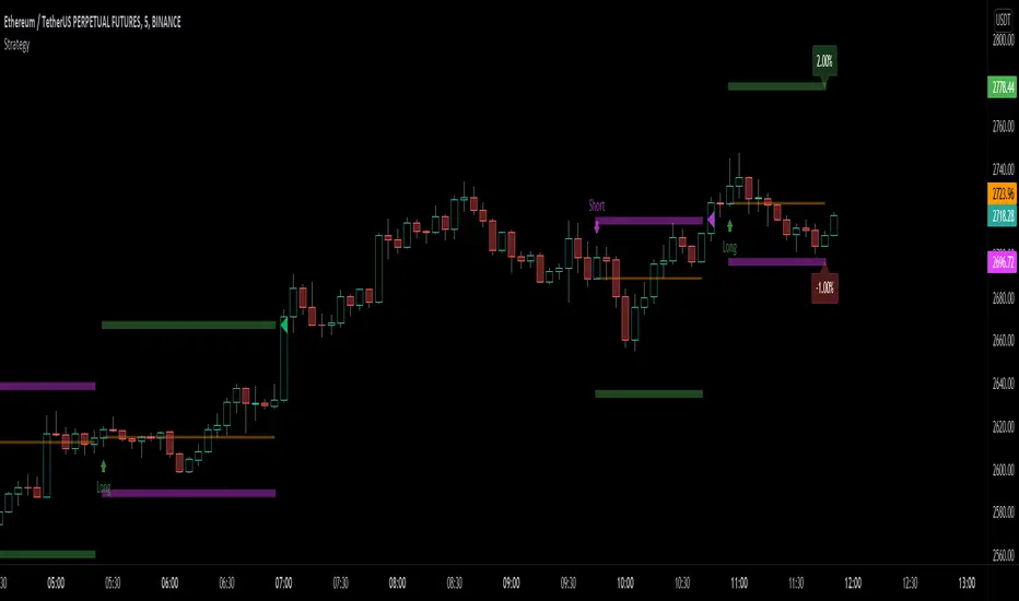
Strategy█ OVERVIEW
This library is a Pine Script™ programmer’s tool containing a variety of strategy-related functions to assist in calculations like profit and loss, stop losses and limits. It also includes several useful functions one can use to convert between units in ticks, price, currency or a percentage of the position's size.
█ CONCEPTS
The library contains three types of functions:
1 — Functions beginning with `percent` take either a portion of a price, or the current position's entry price and convert it to the value outlined in the function's documentation.
Example: Converting a percent of the current position entry price to ticks, or calculating a percent profit at a given level for the position.
2 — Functions beginning with `tick` convert a tick value to another form.
These are useful for calculating a price or currency value from a specified number of ticks.
3 — Functions containing `Level` are used to calculate a stop or take profit level using an offset in ticks from the current entry price.
These functions can be used to plot stop or take profit levels on the chart, or as arguments to the `limit` and `stop` parameters in strategy.exit() function calls.
Note that these calculated levels flip automatically with the position's bias.
For example, using `ticksToStopLevel()` will calculate a stop level under the entry price for a long position, and above the entry price for a short position.
There are also two functions to assist in calculating a position size using the entry's stop and a fixed risk expressed as a percentage of the current account's equity. By varying the position size this way, you ensure that entries with different stop levels risk the same proportion of equity.
█ NOTES
Example code using some of the library's functions is included at the end of the library. To see it in action, copy the library's code to a new script in the Pine Editor, and “Add to chart”.
For each trade, the code displays:
• The entry level in orange.
• The stop level in fuchsia.
• The take profit level in green.
The stop and take profit levels automatically flip sides based on whether the current position is long or short.
Labels near the last trade's levels display the percentages used to calculate them, which can be changed in the script's inputs.
We plot markers for entries and exits because strategy code in libraries does not display the usual markers for them.
Look first. Then leap.
█ FUNCTIONS
percentToTicks(percent) Converts a percentage of the average entry price to ticks.
Parameters:
percent : (series int/float) The percentage of `strategy.position_avg_price` to convert to ticks. 50 is 50% of the entry price.
Returns: (float) A value in ticks.
percentToPrice(percent) Converts a percentage of the average entry price to a price.
Parameters:
percent : (series int/float) The percentage of `strategy.position_avg_price` to convert to price. 50 is 50% of the entry price.
Returns: (float) A value in the symbol's quote currency (USD for BTCUSD).
percentToCurrency(price, percent) Converts the percentage of a price to money.
Parameters:
price : (series int/float) The symbol's price.
percent : (series int/float) The percentage of `price` to calculate.
Returns: (float) A value in the symbol's currency.
percentProfit(exitPrice) Calculates the profit (as a percentage of the position's `strategy.position_avg_price` entry price) if the trade is closed at `exitPrice`.
Parameters:
exitPrice : (series int/float) The potential price to close the position.
Returns: (float) Percentage profit for the current position if closed at the `exitPrice`.
priceToTicks(price) Converts a price to ticks.
Parameters:
price : (series int/float) Price to convert to ticks.
Returns: (float) A quantity of ticks.
ticksToPrice(price) Converts ticks to a price offset from the average entry price.
Parameters:
price : (series int/float) Ticks to convert to a price.
Returns: (float) A price level that has a distance from the entry price equal to the specified number of ticks.
ticksToCurrency(ticks) Converts ticks to money.
Parameters:
ticks : (series int/float) Number of ticks.
Returns: (float) Money amount in the symbol's currency.
ticksToStopLevel(ticks) Calculates a stop loss level using a distance in ticks from the current `strategy.position_avg_price` entry price. This value can be plotted on the chart, or used as an argument to the `stop` parameter of a `strategy.exit()` call. NOTE: The stop level automatically flips based on whether the position is long or short.
Parameters:
ticks : (series int/float) The distance in ticks from the entry price to the stop loss level.
Returns: (float) A stop loss level for the current position.
ticksToTpLevel(ticks) Calculates a take profit level using a distance in ticks from the current `strategy.position_avg_price` entry price. This value can be plotted on the chart, or used as an argument to the `limit` parameter of a `strategy.exit()` call. NOTE: The take profit level automatically flips based on whether the position is long or short.
Parameters:
ticks : (series int/float) The distance in ticks from the entry price to the take profit level.
Returns: (float) A take profit level for the current position.
calcPositionSizeByStopLossTicks(stopLossTicks, riskPercent) Calculates the position size needed to implement a given stop loss (in ticks) corresponding to `riskPercent` of equity.
Parameters:
stopLossTicks : (series int) The stop loss (in ticks) that will be used to protect the position.
riskPercent : (series int/float) The maximum risk level as a percent of current equity (`strategy.equity`).
Returns: (int) A quantity of contracts.
calcPositionSizeByStopLossPercent(stopLossPercent, riskPercent, entryPrice) Calculates the position size needed to implement a given stop loss (%) corresponding to `riskPercent` of equity.
Parameters:
stopLossPercent : (series int/float) The stop loss in percent that will be used to protect the position.
riskPercent : (series int/float) The maximum risk level as a percent of current equity (`strategy.equity`).
entryPrice : (series int/float) The entry price of the position.
Returns: (int) A quantity of contracts.
exitPercent(id, lossPercent, profitPercent, qty, qtyPercent, comment, when, alertMessage) A wrapper of the `strategy.exit()` built-in which adds the possibility to specify loss & profit in as a value in percent. NOTE: this function may work incorrectly with pyramiding turned on due to the use of `strategy.position_avg_price` in its calculations of stop loss and take profit offsets.
Parameters:
id : (series string) The order identifier of the `strategy.exit()` call.
lossPercent : (series int/float) Stop loss as a percent of the entry price.
profitPercent : (series int/float) Take profit as a percent of the entry price.
qty : (series int/float) Number of contracts/shares/lots/units to exit a trade with. The default value is `na`.
qtyPercent : (series int/float) The percent of the position's size to exit a trade with. If `qty` is `na`, the default value of `qty_percent` is 100.
comment : (series string) Optional. Additional notes on the order.
when : (series bool) Condition of the order. The order is placed if it is true.
alertMessage : (series string) An optional parameter which replaces the {{strategy.order.alert_message}} placeholder when it is used in the "Create Alert" dialog box's "Message" field.
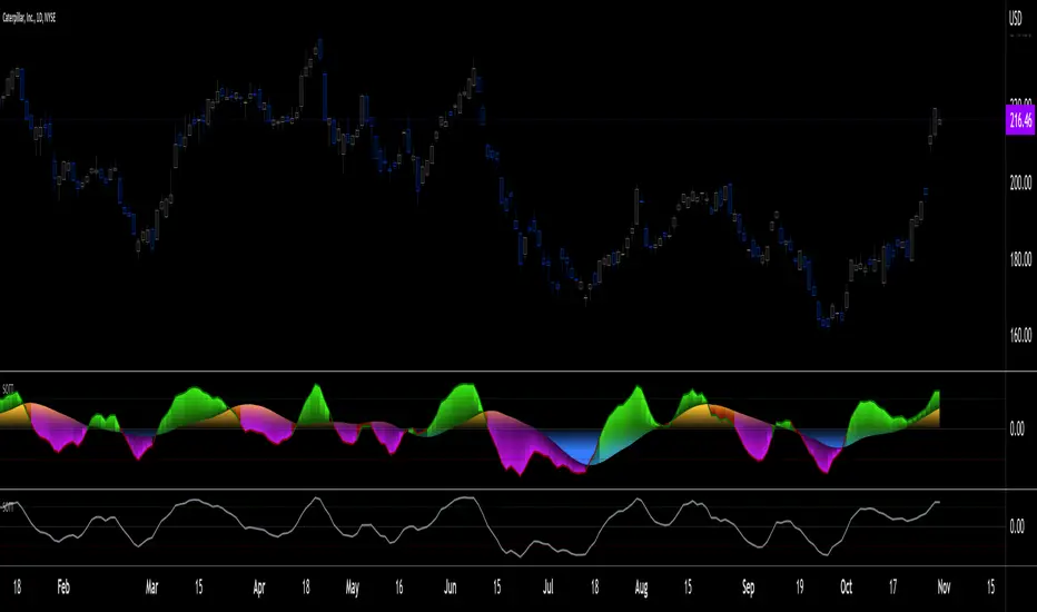
Signs of the Times [LucF]█ OVERVIEW
This oscillator calculates the directional strength of bars using a primitive weighing mechanism based on a small number of what I consider to be fundamental properties of a bar. It does not consider the amplitude of price movements, so can be used as a complement to momentum-based oscillators. It thus belongs to the same family of indicators as my Bar Balance , Volume Ticks , Efficient work , Volume Buoyancy or my Delta Volume indicators.
█ CONCEPTS
The calculations underlying Signs of the Times (SOTT) use a simple, oft-explored concept: measure bar attributes, assign a weight to them, and aggregate results to provide an evaluation of a bar's directional strength. Bull and bear weights are added independently, then subtracted and divided by the maximum possible weight, so the final calculation looks like this:
(up - dn) / weightRange
SOTT has a zero centerline and oscillates between +1 and -1. Ten elementary properties are evaluated. Most carry a weight of one, a few are doubly weighted. All properties are evaluated using only the current bar's values or by comparing its values to those of the preceding bar. The bull conditions follow; their inverse applies to bear conditions:
Weight of 1
• Bar's close is greater than the bar's open (bar is considered to be of "up" polarity)
• Rising open
• Rising high
• Rising low
• Rising close
• Bar is up and its body size is greater than that of the previous bar
• Bar is up and its body size is greater than the combined size of wicks
Weight of 2
• Gap to the upside
• Efficient Work when it is positive
• Bar is up and volume is greater than that of the previous bar (this only kicks in if volume is actually available on the chart's data feed)
Except for the Efficient Work weight, which is a +1 to -1 float value multiplied by 2, all weights are discrete; either zero or the full weight of 1 or 2 is generated. This will cause any gap, for example, to generate a weight of +2 or -2, regardless of the gap's size. That is the reason why the oscillator is oblivious to the amplitude of price movements.
You can see the code used to calculate SOTT in my ta library 's `sott()` function.
█ HOW TO USE THE INDICATOR
No videos explain this indicator and none are planned; reading this description or the script's code is the only way to understand what Signs of the Times does.
Load the indicator on an active chart (see here if you don't know how).
The default configuration displays:
• An Arnaud-Legoux moving average of length 20 of the instant SOTT value. This is the signal line.
• A fill between the MA and the centerline.
• Levels at arbitrary values of +0.3 and -0.3.
• A channel between the signal line and its MA (a simple MA of length 20), which can be one of four colors:
• Bull (green): The signal line is above its MA.
• Strong bull (lime): The bull condition is fulfilled and the signal line is above the centerline.
• Bear (red): The signal line is below its MA.
• Strong bear (pink): The bear condition is fulfilled and the signal line is below the centerline.
The script's "Inputs" tab allows you to:
• Choose a higher timeframe to calculate the indicator's values. This can be useful to get a wider perspective of the indicator's values.
If you elect to use a higher timeframe, make sure that your chart's timeframe is always lower than the higher timeframe you specified,
as calculating on a timeframe lower than the chart's does not make much sense because the indicator is then displaying only the value of the last intrabar in the chart bar.
• Specify the type of MA used to produce the signal line. Use a length of 1 or the Data Window to see the instant value of SOTT. It is quite noisy, thus the need to average it.
• Specify the type of MA applied to the signal line. The idea here is to provide context to the signal.
• Control the display and colors of the lines and fills.
The first pane of this publication's chart shows the default setup. The second one shows only a monochrome signal line.
Using the "Style" tab of the indicator's settings, you can change the type and width of the lines, and the level values.
█ INTERPRETATION
Remember that Signs of the Times evaluates directional bar strength — not price movement. Its highs and lows do not reflect price, but the strength of chart bars. The fact that SOTT knows nothing of how far price moves or of trends is easy to forget. As such, I think SOTT is best used as a confirmation tool. Chart movements may appear to be easy to read when looking at historical bars, but when you have to make go-no-go decisions on the last bar, the landscape often becomes murkier. By providing a quantitative evaluation of the strength of the last few bars, which is not always easily discernible by simply looking at them, SOTT aims to help you decide if the short-term past favors the bets you are considering. Can SOTT predict the future? Of course not.
While SOTT uses completely different calculations than classical momentum oscillators, its profile shares many of their characteristics. This could lead one to infer that directional bar strength correlates with price movement, which could in turn lead one to conclude that indicators such as this one are useless, or that they can be useful tools to confirm momentum oscillators or other models of price movement. The call is, of course, up to you. You can try, for example, to compare a Wilder MA of SOTT to an RSI of the same length.
One key difference with momentum oscillators is that SOTT is much less sensitive to large price movements. The default Arnaud-Legoux MA used for the signal line makes it quite active; you can use a more quiet SMA or EMA if you prefer to tone it down.
In systems where it can be useful to only enter or exit on short-term strength, an average of SOTT values over the last 3 to 5 bars can be used as a more quiet filter than a momentum oscillator would.
█ NOTES
My publications often go through a long gestation period where I use them on my charts or in systems before deciding if they are worth a publication. With an incubation period of more than three years, Signs of the Times holds the record. The properties SOTT currently evaluates result from the systematic elimination of contaminants over that lengthy period of time. It was long because of my usual, slow gear, but also because I had to try countless combinations of conditions before realizing that, contrary to my intuition, best results were achieved by:
• Keeping the number of evaluated properties to the absolute minimum.
• Limiting the evaluation's scope to the current and preceding bar.
• Choosing properties that, in my view, were unmistakably indicative of bullish/bearish conditions.
Repainting
As most oscillators, the indicator provides live realtime values that will recalculate with chart updates. It will thus repaint in real time, but not on historical values. To learn more about repainting, see the Pine Script™ User Manual's page on the subject .
Estimated Time At Price [Kioseff Trading]Hello!
This script uses the same formula as the recently released "Volume Delta" script to ascertain lower timeframe values.
Instead, this script looks to estimate the approximate time spent at price blocks; all time estimates are in minute.second format.
The image above shows functionality. Time spent at price levels/blocks are estimated in duration. The highest estimated block is the highlighted level and a POC line is extended right until violated. Colors, the presence of POC lines and whether they're removed subsequent violation are all configurable.
As show in the image above, the data is displayable in an additional format. When select the "non-classic" format shown above - precise price levels are calculated and the estimated time spent at those levels is summed and displayed right of the current bar. The off-colored level (yellow in the example) denotes the price level encompassing the highest *estimated* time spent.
You can deselect the neon effect and choose to have the script recalculate after any conceivable amount of time has passed.
The script can also calculate for the most current bar should you configure it to do so.
That's all! (for now). A quick/easy script building off an existing foundation.
If you've any ideas for features and ways to "spice up" this script please let me know (: I'll gladly incorporate requests.
Thank you!

Volume Profile, Pivot Anchored by DGTVolume Profile (also known as Price by Volume ) is an charting study that displays trading activity over a specified time period at specific price levels. It is plotted as a horizontal histogram on the finacial isntrumnet's chart that highlights the trader's interest at specific price levels. Specified time period with Pivots Anchored Volume Profile is determined by the Pivot Levels, where the Pivot Points High Low indicator is used and presented with this Custom indicator
Finally, Volume Weighted Colored Bars indicator is presneted with the study
Different perspective of Volume Profile applications;
Anchored to Session, Week, Month etc : Anchored-Volume-Profile
Custom Range, Interactive : Volume-Profile-Custom-Range
Fixed Range with Volume Indicator : Volume-Profile-Fixed-Range
Combined with Support and Resistance Indicator : Price-Action-Support-Resistance and Volume-Profile
Combined with Supply and Demand Zones, Interactive : Supply-Demand-and-Equilibrium-Zones
Disclaimer : Trading success is all about following your trading strategy and the indicators should fit within your trading strategy, and not to be traded upon solely
The script is for informational and educational purposes only. Use of the script does not constitutes professional and/or financial advice. You alone the sole responsibility of evaluating the script output and risks associated with the use of the script. In exchange for using the script, you agree not to hold dgtrd TradingView user liable for any possible claim for damages arising from any decision you make based on use of the script

Fair Value MSThis indicator introduces rigid rules to familiar concepts to better capture and visualize Market Structure and Areas of Support and Resistance in a way that is both rule-based and reactive to market movements.
Typical "Market Structure" or "Zig-Zag" methods determine swing points based on fixed thresholds (length or percentage). While this does provide rigid structure, the results may be lagging or confusing due to the timing, since it is fixed to static parameters.
I believe the concept of Fair Value Gaps can solve this problem.
As you will notice, there are no length settings in this indicator.
> FVG Market Structure
Fair Value Gaps are a well known concept used to indicate directional intent, forming when price moves aggressively in one direction, leaving behind an imbalance between buyers and sellers. While the term FVG was popularized by ICT, the underlying concept predates them, known historically as imbalances, inefficiencies, or liquidity voids in institutional trading.
Note: For simplicity, in this indicator they'll be called FVGs.
By reading into this, we are able to clearly and rigidly define market structure simply by "looking" at the chart, using objective price events rather than subjective interpretation, or lengths.
By using FVGs to determine structure direction, the length, and speed of identification lies entirely on the market. If an FVG Down occurs immediately after a New Higher High forms, it is reasonable to assume there was a seller at that point, so the script would indicate a New Swing High.
The script is NOT stuck, waiting for a % retrace, or # bars to pass to identify it as such.
Sometimes the market is in a steady trend in a single direction and no FVGs form; therefore, no structure forms. -> Why would we try to impose structure on a clear trend?
Ultimately, the FVG Structure Method uses real reactions from the market to determine Market structure, and is not fixed to specific parameters.
As with other market structure indicators, "Market Structure Breaks" are still identifiable when price moves outside the most recent swing points.
These are helpful to indicate larger direction. In the following section you will see how these help us determine when we should start the search for an "Area of Interest (AOI)".
> Areas of Interest (AOIs)
"Area of Interest (AOI)" is a generalized term, and could refer to many types of zones you might recognize under different names. While the AOIs in this indicator are specialized in their own way, I have chosen to simply use the term "Area of Interest" because it’s more important to understand how they behave and why they exist than to focus on what they’re called.
The goal of an AOI is to point out reasonable areas where buyers or sellers may be staging, as is typical with support and resistance.
In order to reasonably identify these areas, we look for cause and effect relationships. When considering these relationships, it's easier to understand the placement of the points to define each zone.
(Buyer Examples)
Cause: Strong Buyers step in at Swing Low
Effect: Fair Value Gap Forms
Cause: Sustained Buying Pressure
Effect: Market Structure Breaks
In this example, The zone is drawn from the Swing Low, to the Bottom of the FVG closest to the swing point.
In theory, the participation at the swing point was strong and aggressive enough to create the FVG imbalance. Which then found acceptance and continued into a Market Structure Break. So with these AOIs, we are trying to locate the aggressive Buyers or Sellers which were positioned BEFORE the FVG.
These Zones are intended to act as areas to look for reactions from market participants, to judge where price may be going. When revisiting these zones, we look for a reaction or a break, to further provide us information to if the buyers or sellers are still there.
As seen in the screenshot above, The information we gain is not from the creation of these zones, but from the behavior we witness when these zones are revisited.
Technical Note: In this indicator, Market Structure Breaks are only considered when price closes outside the recent swing points. Wicks are not considered as confirmation, therefore are not used to detect structural breaks.
Inside each AOI you can optionally display a readout of the volume which accumulated during the time starting at the swing point and going until the closing bar of the FVG.
Note: We are counting volume until the closing bar of the FVG since the FVG is a 3 bar formation, and aggressive volume is required throughout to create the imbalance.
There are multiple FVGs that typically occur in a single direction, but we do not look to every single one to be indicative of structure, only the first FVG in the opposite direction of the previous direction (which is determined by previous FVGs)
You will probably notice, the AOIs do not form from the closest swing or FVG to the break, this is because we are targeting larger directional changes to draw these AOIs from.
Since they do not always happen perfectly every time, the AOI formation waits for an FVG to occur AND a Market structure break to happen. One without the other will result in no Zone displaying.
> Reflection Lines
While they may seem slightly redundant, Reflection Lines serve as reminders of previous support and resistance pivots. They are drawn at the same Pivots where and AOI is formed, and extend beyond the mitigation of the AOI.
These lines are often points of price to look for "Support Flips", a re-test pattern where price trades through previous support (or resistance) then returns to it and rejects, continuing into a larger move or trend.
Their namesake is based on the behavior of price, "reflecting" at these levels.
The Reflection lines are simple and change color based on price's location.
If price is above, we would typically look to a reflection line in with support in mind.
As a basic filter, these lines use an average price to determine their color, this way they will not change their color as frequently in choppy situations.
> Session Start/End Lines
For analysis purposes and trade review, it is helpful to analyze with context.
For that reason, I have implemented start and end session lines into the indicator, these are helpful when reviewing historical charts to not provide additional context.
By default, they are set to the NYSE Session, but can be changed to fit any needs.
These lines are not advanced, and simply draw a line as the chart passes the start and end of the sessions. It's very likely that you may need to adjust the session for your specific needs.
Note: The Timezone can be adjusted within the code if needed. By Default, the indicator uses "America/New_York" Timezone.
> Conclusion
If you’ve ever felt like your structure tools were confusing or lagging, drawing zones too late, or zones that simply don't make sense, this should feel like a breath of fresh air.
By removing arbitrary length settings and instead using FVGs to define structure and as a basis for AOIs, you're getting a more accurate look at what price is doing and where it's reacting from.
This indicator is rule-based, reactive, and aims to keep things logical without fluff or false confidence.
Enjoy!

TextLibrary "Text"
library to format text in different fonts or cases plus a sort function.
🔸 Credits and Usage
This library is inspired by the work of three authors (in chronological order of publication date):
Unicode font function - JD - Duyck
UnicodeReplacementFunction - wlhm
font - kaigouthro
🔹 Fonts
Besides extra added font options, the toFont(fromText, font) method uses a different technique. On the first runtime bar (whether it is barstate.isfirst , barstate.islast , or between) regular letters and numbers and mapped with the chosen font. After this, each character is replaced using the build-in key - value pair map function .
Also an enum Efont is included.
Note: Some fonts are not complete, for example there isn't a replacement for every character in Superscript/Subscript.
Example of usage (besides the included table example):
import fikira/Text/1 as t
i_font = input.enum(t.Efont.Blocks)
if barstate.islast
sentence = "this sentence contains words"
label.new(bar_index, 0, t.toFont(fromText = sentence, font = str.tostring(i_font)), style=label.style_label_lower_right)
label.new(bar_index, 0, t.toFont(fromText = sentence, font = "Circled" ), style=label.style_label_lower_left )
label.new(bar_index, 0, t.toFont(fromText = sentence, font = "Wiggly" ), style=label.style_label_upper_right)
label.new(bar_index, 0, t.toFont(fromText = sentence, font = "Upside Latin" ), style=label.style_label_upper_left )
🔹 Cases
The script includes a toCase(fromText, case) method to transform text into snake_case, UPPER SNAKE_CASE, kebab-case, camelCase or PascalCase, as well as an enum Ecase .
Example of usage (besides the included table example):
import fikira/Text/1 as t
i_case = input.enum(t.Ecase.camel)
if barstate.islast
sentence = "this sentence contains words"
label.new(bar_index, 0, t.toCase(fromText = sentence, case = str.tostring(i_case)), style=label.style_label_lower_right)
label.new(bar_index, 0, t.toCase(fromText = sentence, case = "snake_case" ), style=label.style_label_lower_left )
label.new(bar_index, 0, t.toCase(fromText = sentence, case = "PascalCase" ), style=label.style_label_upper_right)
label.new(bar_index, 0, t.toCase(fromText = sentence, case = "SNAKE_CASE" ), style=label.style_label_upper_left )
🔹 Sort
The sort(strings, order, sortByUnicodeDecimalNumbers) method returns a sorted array of strings.
strings: array of strings, for example words = array.from("Aword", "beyond", "Space", "salt", "pepper", "swing", "someThing", "otherThing", "12345", "_firstWord")
order: "asc" / "desc" (ascending / descending)
sortByUnicodeDecimalNumbers: true/false; default = false
_____
• sortByUnicodeDecimalNumbers: every Unicode character is linked to a Unicode Decimal number ( wikipedia.org/wiki/List_of_Unicode_characters ), for example:
1 49
2 50
3 51
...
A 65
B 66
...
S 83
...
_ 95
` 96
a 97
b 98
...
o 111
p 112
q 113
r 114
s 115
...
This means, if we sort without adjusting ( sortByUnicodeDecimalNumbers = true ), in ascending order, the letter b (98 - small) would be after S (83 - Capital).
By disabling sortByUnicodeDecimalNumbers , Capital letters are intermediate transformed to str.lower() after which the Unicode Decimal number is retrieved from the small number instead of the capital number. For example S (83) -> s (115), after which the number 115 is used to sort instead of 83.
Example of usage (besides the included table example):
import fikira/Text/1 as t
if barstate.islast
aWords = array.from("Aword", "beyond", "Space", "salt", "pepper", "swing", "someThing", "otherThing", "12345", "_firstWord")
label.new(bar_index, 0, str.tostring(t.sort(strings= aWords, order = 'asc' , sortByUnicodeDecimalNumbers = false)), style=label.style_label_lower_right)
label.new(bar_index, 0, str.tostring(t.sort(strings= aWords, order = 'desc', sortByUnicodeDecimalNumbers = false)), style=label.style_label_lower_left )
label.new(bar_index, 0, str.tostring(t.sort(strings= aWords, order = 'asc' , sortByUnicodeDecimalNumbers = true )), style=label.style_label_upper_right)
label.new(bar_index, 0, str.tostring(t.sort(strings= aWords, order = 'desc', sortByUnicodeDecimalNumbers = true )), style=label.style_label_upper_left )
🔸 Methods/functions
method toFont(fromText, font)
toFont : Transforms text into the selected font
Namespace types: series string, simple string, input string, const string
Parameters:
fromText (string)
font (string)
Returns: `fromText` transformed to desired `font`
method toCase(fromText, case)
toCase : formats text to snake_case, UPPER SNAKE_CASE, kebab-case, camelCase or PascalCase
Namespace types: series string, simple string, input string, const string
Parameters:
fromText (string)
case (string)
Returns: `fromText` formatted to desired `case`
method sort(strings, order, sortByUnicodeDecimalNumbers)
sort : sorts an array of strings, ascending/descending and by Unicode Decimal numbers or not.
Namespace types: array
Parameters:
strings (array)
order (string)
sortByUnicodeDecimalNumbers (bool)
Returns: Sorted array of strings

Risk Distribution HistogramStatistical risk visualization and analysis tool for any ticker 📊
The Risk Distribution Histogram visualizes the statistical distribution of different risk metrics for any financial instrument. It converts risk data into histograms with quartile-based color coding, so that traders can understand their risk, tail-risks, exposure patterns and make data-driven decisions based on empirical evidence rather than assumptions.
The indicator supports multiple risk calculation methods, each designed for different aspects of market analysis, from general volatility assessment to tail risk analysis.
Risk Measurement Methods
Standard Deviation
Captures raw daily price volatility by measuring the dispersion of price movements. Ideal for understanding overall market conditions and timing volatility-based strategies.
Use case: Options trading and volatility analysis.
Average True Range (ATR)
Measures true range as a percentage of price, accounting for gaps and limit moves. Valuable for position sizing across different price levels.
Use case: Position sizing and stop-loss placement.
The chart above illustrates how ATR statistical distribution can be used by looking at the ATR % of price distribution. For example, 90% of the movements are below 5%.
Downside Deviation
Only considers negative price movements, making it ideal for checking downside risk and capital protection rather than capturing upside volatility.
Use case: Downside protection strategies and stop losses.
Drawdown Analysis
Tracks peak-to-trough declines, providing insight into maximum loss potential during different market conditions.
Use case: Risk management and capital preservation.
The chart above illustrates tale risk for the asset (TQQQ), showing that it is possible to have drawdowns higher than 20%.
Entropy-Based Risk (EVaR)
Uses information theory to quantify market uncertainty. Higher entropy values indicate more unpredictable price action, valuable for detecting regime changes.
Use case: Advanced risk modeling and tail-risk.
VIX Histogram
Incorporates the market's fear index directly into analysis, showing how current volatility expectations compare to historical patterns. The CAPITALCOM:VIX histogram is independent from the ticker on the chart.
Use case: Volatility trading and market timing.
Visual Features
The histogram uses quartile-based color coding that immediately shows where current risk levels stand relative to historical patterns:
Green (Q1): Low Risk (0-25th percentile)
Yellow (Q2): Medium-Low Risk (25-50th percentile)
Orange (Q3): Medium-High Risk (50-75th percentile)
Red (Q4): High Risk (75-100th percentile)
The data table provides detailed statistics, including:
Count Distribution: Historical observations in each bin
PMF: Percentage probability for each risk level
CDF: Cumulative probability up to each level
Current Risk Marker: Shows your current position in the distribution
Trading Applications
When current risk falls into upper quartiles (Q3 or Q4), it signals conditions are riskier than 50-75% of historical observations. This guides position sizing and portfolio adjustments.
Key applications:
Position sizing based on empirical risk distributions
Monitoring risk regime changes over time
Comparing risk patterns across timeframes
Risk distribution analysis improves trade timing by identifying when market conditions favor specific strategies.
Enter positions during low-risk periods (Q1)
Reduce exposure in high-risk periods (Q4)
Use percentile rankings for dynamic stop-loss placement
Time volatility strategies using distribution patterns
Detect regime shifts through distribution changes
Compare current conditions to historical benchmarks
Identify outlier events in tail regions
Validate quantitative models with empirical data
Configuration Options
Data Collection
Lookback Period: Control amount of historical data analyzed
Date Range Filtering: Focus on specific market periods
Sample Size Validation: Automatic reliability warnings
Histogram Customization
Bin Count: 10-50 bins for different detail levels
Auto/Manual Bin Width: Optimize for your data range
Visual Preferences: Custom colors and font sizes
Implementation Guide
Start with Standard Deviation on daily charts for the most intuitive introduction to distribution-based risk analysis.
Method Selection: Begin with Standard Deviation
Setup: Use daily charts with 20-30 bins
Interpretation: Focus on quartile transitions as signals
Monitoring: Track distribution changes for regime detection
The tool provides comprehensive statistics including mean, standard deviation, quartiles, and current position metrics like Z-score and percentile ranking.
Enjoy, and please let me know your feedback! 😊🥂

Crowding model ║ BullVision🔬 Overview
The Crypto Crowding Model Pro is a sophisticated analytical tool designed to visualize and quantify market conditions across multiple cryptocurrencies. By leveraging Relative Strength Index (RSI) and Z-score calculations, this indicator provides traders with an intuitive and detailed snapshot of current crypto market dynamics, highlighting areas of extreme momentum, crowded trades, and potential reversal points.
⚙️ Key Concepts
📊 RSI and Z-Score Analysis
RSI (Relative Strength Index) evaluates the momentum and strength of each cryptocurrency, identifying overbought or oversold conditions.
Z-Score Normalization measures each asset's current price deviation relative to its historical average, identifying statistically significant extremes.
🎯 Crowding Analytics
An integrated analytics panel provides real-time crowding metrics, quantifying market sentiment into four distinct categories:
🔥 FOMO (Fear of Missing Out): High momentum, potential exhaustion.
❄️ Fear: Low momentum, potential reversal or consolidation.
📈 Recovery: Moderate upward momentum after a downward trend.
💪 Strength: Stable bullish conditions with sustained momentum.
🖥️ Visual Scatter Plot
Assets are plotted on a dynamic scatter plot, positioning each cryptocurrency according to its RSI and Z-score.
Color coding, symbol shapes, and sizes help quickly identify main market segments (BTC, ETH, TOTAL, OTHERS) and individual asset conditions.
🧩 Quadrant Classification
Assets are categorized into four quadrants based on their momentum and deviation:
Overbought Extended: High RSI and positive Z-score.
Recovery Phase: Low RSI but positive Z-score.
Oversold Compressed: Low RSI and negative Z-score.
Strong Consolidation: High RSI but negative Z-score.
🔧 User Customization
🎨 Visual Settings
Bar Scale: Adjust the scatter plot visual scale.
Asset Visibility: Optionally display key market benchmarks (TOTAL, BTC, ETH, OTHERS).
Gradient Background: Enhances visual interpretation of asset clusters.
Crowding Analytics Panel: Toggle the analytics panel on/off.
📊 Indicator Parameters
RSI Length: Defines the calculation period for RSI.
Z-score Lookback: Historical lookback period for normalization.
Crowding Alert Threshold: Sets alert sensitivity for crowded market conditions.
🎯 Zone Settings
Quadrant Labels: Displays descriptive labels for each quadrant.
Danger Zones: Highlights extreme RSI levels indicative of heightened market risk.
📈 Visual Output
Dynamic Scatter Plot: Visualizes asset positioning clearly and intuitively.
Gradient and Grid: Professional gridlines and subtle gradient backgrounds assist visual assessment.
Danger Zone Highlights: Visually indicates RSI extremes to warn of potential market turning points.
Crowding Analytics Panel: Real-time summary of market sentiment and asset distribution.
🔍 Use Cases
This indicator is particularly beneficial for traders and analysts looking to:
Identify crowded trades and potential reversal points.
Quickly assess overall market sentiment and individual asset strength.
Integrate a robust momentum analysis into broader technical or fundamental strategies.
Enhance market timing and improve risk management decisions.
⚠️ Important Notes
This indicator does not provide explicit buy or sell signals.
It is intended solely for informational, analytical, and educational purposes.
Past performance and signals are not indicative of future market results.
Always combine with additional tools and analysis as part of comprehensive decision-making.

Dynamic Gap Probability ToolDynamic Gap Probability Tool measures the percentage gap between price and a chosen moving average, then analyzes your chart history to estimate the likelihood of the next candle moving up or down. It dynamically adjusts its sample size to ensure statistical robustness while focusing on the exact deviation level.
Originality and Value:
• Combines gap-based analysis with dynamic sample aggregation to balance precision and reliability.
• Automatically extends the sample when exact matches are scarce, avoiding misleading signals on rare extreme moves.
• Provides real “next-candle” probabilities based on historical occurrences rather than fixed thresholds or untested heuristics.
• Adds value by giving traders an evidence-based edge: you see how similar past deviations actually played out.
How It Works:
1. Calculate gap = (close – moving average) / moving average * 100.
2. Round the absolute gap to nearest percent (X%).
3. Count historical bars where gap ≥ X% above or ≤ –X% below.
4. If exact X% count is below the minimum occurrences threshold, include gaps at X+1%, X+2%, etc., until threshold is reached.
5. Compute “next-candle” green vs. red probabilities from the aggregated sample.
6. Display current gap, sample size, green probability, and red probability in a table.
Inputs:
• Moving Average Type (SMA, EMA, WMA, VWMA, HMA, SMMA, TMA)
• Moving Average Period (default 200)
• Minimum Occurrences Threshold (default 50)
• Table position and styling options
Examples:
• If price is 3% above the 200-period SMA and 120 occurrences ≥3% are found, with 84 green next candles (70%) and 36 red (30%), the script displays “3% | 120 | 70% green | 30% red.”
• If price is 8% below the SMA but only 20 exact matches exist, the script will include 9% and 10% gaps until it reaches 50 samples, then calculate probabilities from that broader set.
Why It’s Useful:
• Mean-reversion traders see green-probability signals at extreme overbought or oversold levels.
• Trend-followers identify continuation likelihood when red probability is high.
• Risk managers gauge reliability by inspecting sample size before acting on any signal.
Limitations:
• Historical probabilities do not guarantee future performance.
• Results depend on timeframe and symbol, backtest with your data before trading.
• Use realistic slippage and commission when overlaying on strategy scripts.

EVaR Indicator and Position SizingThe Problem:
Financial markets consistently show "fat-tailed" distributions where extreme events occur with higher frequency than predicted by normal distributions (Gaussian or even log-normal). These fat tails manifest in sudden price crashes, volatility spikes, and black swan events that traditional risk measures like volatility can underestimate. Standard deviation and conventional VaR calculations assume normally distributed returns, leaving traders vulnerable to severe drawdowns during market stress.
Cryptocurrencies and volatile instruments display particularly pronounced fat-tailed behavior, with extreme moves occurring 5-10 times more frequently than normal distribution models would predict. This reality demands a more sophisticated approach to risk measurement and position sizing.
The Solution: Entropic Value at Risk (EVAR)
EVaR addresses these limitations by incorporating principles from statistical mechanics and information theory through Tsallis entropy. This advanced approach captures the non-linear dependencies and power-law distributions characteristic of real financial markets.
Entropy is more adaptive than standard deviations and volatility measures.
I was inspired to create this indicator after reading the paper " The End of Mean-Variance? Tsallis Entropy Revolutionises Portfolio Optimisation in Cryptocurrencies " by by Sana Gaied Chortane and Kamel Naoui.
Key advantages of EVAR over traditional risk measures:
Superior tail risk capture: More accurately quantifies the probability of extreme market moves
Adaptability to market regimes: Self-calibrates to changing volatility environments
Non-parametric flexibility: Makes less assumptions about the underlying return distribution
Forward-looking risk assessment: Better anticipates potential market changes (just look at the charts :)
Mathematically, EVAR is defined as:
EVAR_α(X) = inf_{z>0} {z * log(1/α * M_X(1/z))}
Where the moment-generating function is calculated using q-exponentials rather than conventional exponentials, allowing precise modeling of fat-tailed behavior.
Technical Implementation
This indicator implements EVAR through a q-exponential approach from Tsallis statistics:
Returns Calculation: Price returns are calculated over the lookback period
Moment Generating Function: Approximated using q-exponentials to account for fat tails
EVAR Computation: Derived from the MGF and confidence parameter
Normalization: Scaled to for intuitive visualization
Position Sizing: Inversely modulated based on normalized EVAR
The q-parameter controls tail sensitivity—higher values (1.5-2.0) increase the weighting of extreme events in the calculation, making the model more conservative during potentially turbulent conditions.
Indicator Components
1. EVAR Risk Visualization
Dynamic EVAR Plot: Color-coded from red to green normalized risk measurement (0-1)
Risk Thresholds: Reference lines at 0.3, 0.5, and 0.7 delineating risk zones
2. Position Sizing Matrix
Risk Assessment: Current risk level and raw EVAR value
Position Recommendations: Percentage allocation, dollar value, and quantity
Stop Parameters: Mathematically derived stop price with percentage distance
Drawdown Projection: Maximum theoretical loss if stop is triggered
Interpretation and Application
The normalized EVAR reading provides a probabilistic risk assessment:
< 0.3: Low risk environment with minimal tail concerns
0.3-0.5: Moderate risk with standard tail behavior
0.5-0.7: Elevated risk with increased probability of significant moves
> 0.7: High risk environment with substantial tail risk present
Position sizing is automatically calculated using an inverse relationship to EVAR, contracting during high-risk periods and expanding during low-risk conditions. This is a counter-cyclical approach that ensures consistent risk exposure across varying market regimes, especially when the market is hyped or overheated.
Parameter Optimization
For optimal risk assessment across market conditions:
Lookback Period: Determines the historical window for risk calculation
Q Parameter: Controls tail sensitivity (higher values increase conservatism)
Confidence Level: Sets the statistical threshold for risk assessment
For cryptocurrencies and highly volatile instruments, a q-parameter between 1.5-2.0 typically provides the most accurate risk assessment because it helps capturing the fat-tailed behavior characteristic of these markets. You can also increase the q-parameter for more conservative approaches.
Practical Applications
Adaptive Risk Management: Quantify and respond to changing tail risk conditions
Volatility-Normalized Positioning: Maintain consistent exposure across market regimes
Black Swan Detection: Early identification of potential extreme market conditions
Portfolio Construction: Apply consistent risk-based sizing across diverse instruments
This indicator is my own approach to entropy-based risk measures as an alterative to volatility and standard deviations and it helps with fat-tailed markets.
Enjoy!

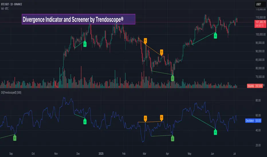
Divergence Screener [Trendoscope®]🎲Overview
The Divergence Screener is a powerful TradingView indicator designed to detect and visualize bullish and bearish divergences, including hidden divergences, between price action and a user-selected oscillator. Built with flexibility in mind, it allows traders to customize the oscillator type, trend detection method, and other parameters to suit various trading strategies. The indicator is non-overlay, displaying divergence signals directly on the oscillator plot, with visual cues such as lines and labels on the chart for easy identification.
This indicator is ideal for traders seeking to identify potential reversal or continuation signals based on price-oscillator divergences. It supports multiple oscillators, trend detection methods, and alert configurations, making it versatile for different markets and timeframes.
🎲Features
🎯Customizable Oscillator Selection
Built-in Oscillators : Choose from a variety of oscillators including RSI, CCI, CMO, COG, MFI, ROC, Stochastic, and WPR.
External Oscillator Support : Users can input an external oscillator source, allowing integration with custom or third-party indicators.
Configurable Length : Adjust the oscillator’s period (e.g., 14 for RSI) to fine-tune sensitivity.
🎯Divergence Detection
The screener identifies four types of divergences:
Bullish Divergence : Price forms a lower low, but the oscillator forms a higher low, signaling potential upward reversal.
Bearish Divergence : Price forms a higher high, but the oscillator forms a lower high, indicating potential downward reversal.
Bullish Hidden Divergence : Price forms a higher low, but the oscillator forms a lower low, suggesting trend continuation in an uptrend.
Bearish Hidden Divergence : Price forms a lower high, but the oscillator forms a higher high, suggesting trend continuation in a downtrend.
🎯Flexible Trend Detection
The indicator offers three methods to determine the trend context for divergence detection:
Zigzag : Uses zigzag pivots to identify trends based on higher highs (HH), higher lows (HL), lower highs (LH), and lower lows (LL).
MA Difference : Calculates the trend based on the difference in a moving average (e.g., SMA, EMA) between divergence pivots.
External Trend Signal : Allows users to input an external trend signal (positive for uptrend, negative for downtrend) for custom trend analysis.
🎯Zigzag-Based Pivot Analysis
Customizable Zigzag Length : Adjust the zigzag length (default: 13) to control the sensitivity of pivot detection.
Repaint Option : Choose whether divergence lines repaint based on the latest data or wait for confirmed pivots, balancing responsiveness and reliability.
🎯Visual and Alert Features
Divergence Visualization : Divergence lines are drawn between price pivots and oscillator pivots, color-coded for easy identification:
Bullish Divergence : Green
Bearish Divergence : Red
Bullish Hidden Divergence : Lime
Bearish Hidden Divergence : Orange
Labels and Tooltips : Labels (e.g., “D” for divergence, “H” for hidden) appear on price and oscillator pivots, with tooltips providing detailed information such as price/oscillator values, ratios, and pivot directions.
Alerts : Configurable alerts for each divergence type (bullish, bearish, bullish hidden, bearish hidden) trigger on bar close, ensuring timely notifications.
🎲 How It Works
🎯Oscillator Calculation
The indicator calculates the selected oscillator (or uses an external source) and plots it on the chart.
Oscillator values are stored in a map for reference during divergence calculations.
🎯Pivot Detection
A zigzag algorithm identifies pivots in the oscillator data, with configurable length and repainting options.
Price and oscillator pivots are compared to detect divergences based on their direction and ratio.
🎯Divergence Identification
The indicator compares price and oscillator pivot directions (HH, HL, LH, LL) to identify divergences.
Trend context is determined using the selected method (Zigzag, MA Difference, or External).
Divergences are classified as bullish, bearish, bullish hidden, or bearish hidden based on price-oscillator relationships and trend direction.
🎯Visualization and Alerts
Valid divergences are drawn as lines connecting price and oscillator pivots, with corresponding labels.
Alerts are triggered for allowed divergence types, providing detailed information via tooltips.
🎯Validation
Divergence lines are validated to ensure no intermediate bars violate the divergence condition, enhancing signal reliability.
🎲 Usage Instructions as Indicator
🎯Add to Chart:
Add the “Divergence Screener ” to your TradingView chart.
The indicator appears in a separate pane below the price chart, plotting the oscillator and divergence signals.
🎯Configure Settings:
Adjust the oscillator type and length to match your trading style.
Select a trend detection method and configure related parameters (e.g., MA type/length or external signal).
Set the zigzag length and repainting preference.
Enable/disable alerts for specific divergence types.
I🎯nterpret Signals:
Bullish Divergence (Green) : Look for potential buy opportunities in a downtrend.
Bearish Divergence (Red) : Consider sell opportunities in an uptrend.
Bullish Hidden Divergence (Lime) : Confirm continuation in an uptrend.
Bearish Hidden Divergence (Orange): Confirm continuation in a downtrend.
Use tooltips on labels to review detailed pivot and divergence information.
🎯Set Alerts:
Create alerts for each divergence type to receive notifications via TradingView’s alert system.
Alerts include detailed text with price, oscillator, and divergence information.
🎲 Example Scenarios as Indicator
🎯 With External Oscillator (Use MACD Histogram as Oscillator)
In order to use MACD as an oscillator for divergence signal instead of the built in options, follow these steps.
Load MACD Indicator from Indicator library
From Indicator settings of Divergence Screener, set Use External Oscillator and select MACD Histograme from the dropdown
You can now see that the oscillator pane shows the data of selected MACD histogram and divergence signals are generated based on the external MACD histogram data.
🎯 With External Trend Signal (Supertrend Ladder ATR)
Now let's demonstrate how to use external direction signals using Supertrend Ladder ATR indicator. Please note that in order to use the indicator as trend source, the indicator should return positive integer for uptrend and negative integer for downtrend. Steps are as follows:
Load the desired trend indicator. In this example, we are using Supertrend Ladder ATR
From the settings of Divergence Screener, select "External" as Trend Detection Method
Select the trend detection plot Direction from the dropdown. You can now see that the divergence signals will rely on the new trend settings rather than the built in options.
🎲 Using the Script with Pine Screener
The primary purpose of the Divergence Screener is to enable traders to scan multiple instruments (e.g., stocks, ETFs, forex pairs) for divergence signals using TradingView’s Pine Screener, facilitating efficient comparison and identification of trading opportunities.
To use the Divergence Screener as a screener, follow these steps:
Add to Favorites : Add the Divergence Screener to your TradingView favorites to make it available in the Pine Screener.
Create a Watchlist : Build a watchlist containing the instruments (e.g., stocks, ETFs, or forex pairs) you want to scan for divergences.
Access Pine Screener : Navigate to the Pine Screener via TradingView’s main menu: Products -> Screeners -> Pine, or directly visit tradingview.com/pine-screener/.
Select Watchlist : Choose the watchlist you created from the Watchlist dropdown in the Pine Screener interface.
Choose Indicator : Select Divergence Screener from the Choose Indicator dropdown.
Configure Settings : Set the desired timeframe (e.g., 1 hour, 1 day) and adjust indicator settings such as oscillator type, zigzag length, or trend detection method as needed.
Select Filter Criteria : Select the condition on which the watchlist items needs to be filtered. Filtering can only be done on the plots defined in the script.
Run Scan : Press the Scan button to display divergence signals across the selected instruments. The screener will show which instruments exhibit bullish, bearish, bullish hidden, or bearish hidden divergences based on the configured settings.
🎲 Limitations and Possible Future Enhancements
Limitations are
Custom input for oscillator and trend detection cannot be used in pine screener.
Pine screener has max 500 bars available.
Repaint option is by default enabled. When in repaint mode expect the early signal but the signals are prone to repaint.
Possible future enhancements
Add more built-in options for oscillators and trend detection methods so that dependency on external indicators is limited
Multi level zigzag support
Logarithmic Moving Average (LMA) [QuantAlgo]🟢 Overview
The Logarithmic Moving Average (LMA) uses advanced logarithmic weighting to create a dynamic trend-following indicator that prioritizes recent price action while maintaining statistical significance. Unlike traditional moving averages that use linear or exponential weights, this indicator employs logarithmic decay functions to create a more sophisticated price averaging system that adapts to market volatility and momentum conditions.
The indicator displays a smoothed signal line that oscillates around zero, with positive values indicating bullish momentum and negative values indicating bearish momentum. The signal incorporates trend quality assessment, momentum confirmation, and multiple filtering mechanisms to help traders and investors identify trend continuation and reversal opportunities across different timeframes and asset classes.
🟢 How It Works
The indicator's core innovation lies in its logarithmic weighting system, where weights are calculated using the formula: w = 1.0 / math.pow(math.log(i + steepness), 2) The steepness parameter controls how aggressively recent data is prioritized over historical data, creating a dynamic weight decay that can be fine-tuned for different trading styles. This logarithmic approach provides more nuanced weight distribution compared to exponential moving averages, offering better responsiveness while maintaining stability.
The LMA calculation combines multiple sophisticated components. First, it calculates the logarithmic weighted average of closing prices. Then it measures the slope of this average over a 10-period lookback: lmaSlope = (lma - lma ) / lma * 100 The system also incorporates trend quality assessment using R-squared correlation analysis of log-transformed prices, measuring how well the price data fits a linear trend model over the specified period.
The final signal generation uses the formula: signal = lmaSlope * (0.5 + rSquared * 0.5) which combines the LMA slope with trend quality weighting. When momentum confirmation is enabled, the indicator calculates annualized log-return momentum and applies a multiplier when the momentum direction aligns with the signal direction, strengthening confirmed signals while filtering out weak or counter-trend movements.
🟢 How to Use
1. Signal Interpretation and Threshold Zones
Positive Values (Above Zero): LMA slope indicating bullish momentum with upward price trajectory relative to logarithmic baseline
Negative Values (Below Zero): LMA slope indicating bearish momentum with downward price trajectory relative to logarithmic baseline
Zero Line Crosses: Signal transitions between bullish and bearish regimes, indicating potential trend changes
Long Entry Threshold Zone: Area above positive threshold (default 0.5) indicating confirmed bullish signals suitable for long positions
Short Entry Threshold Zone: Area below negative threshold (default -0.5) indicating confirmed bearish signals suitable for short positions
Extreme Values: Signals exceeding ±1.0 represent strong momentum conditions with higher probability of continuation
2. Momentum Confirmation and Visual Analysis
Signal Color Intensity: Gradient coloring shows signal strength, with brighter colors indicating stronger momentum
Bar Coloring: Optional price bar coloring matches signal direction for quick visual trend identification
Position Labels: Real-time position classification (Bullish/Bearish/Neutral) displayed on the latest bar
Momentum Weight Factor: When short-term log-return momentum aligns with LMA signal direction, the signal receives additional weight confirmation
Trend Quality Component: R-squared values weight the signal strength, with higher correlation indicating more reliable trend conditions
3. Examples: Preconfigured Settings
Default: Universally applicable configuration balanced for medium-term investing and general trading across multiple timeframes and asset classes.
Scalping: Highly responsive setup with shorter period and higher steepness for ultra-short-term trades on 1-15 minute charts, optimized for quick momentum shifts.
Swing Trading: Extended period with moderate steepness and increased smoothing for multi-day positions, designed to filter noise while capturing larger price swings on 1-4 hour and daily charts.
Trend Following: Maximum smoothing with lower steepness for established trend identification, generating fewer but more reliable signals optimal for daily and weekly timeframes.
Mean Reversion: Shorter period with high steepness for counter-trend strategies, more sensitive to extreme moves and reversal opportunities in ranging market conditions.
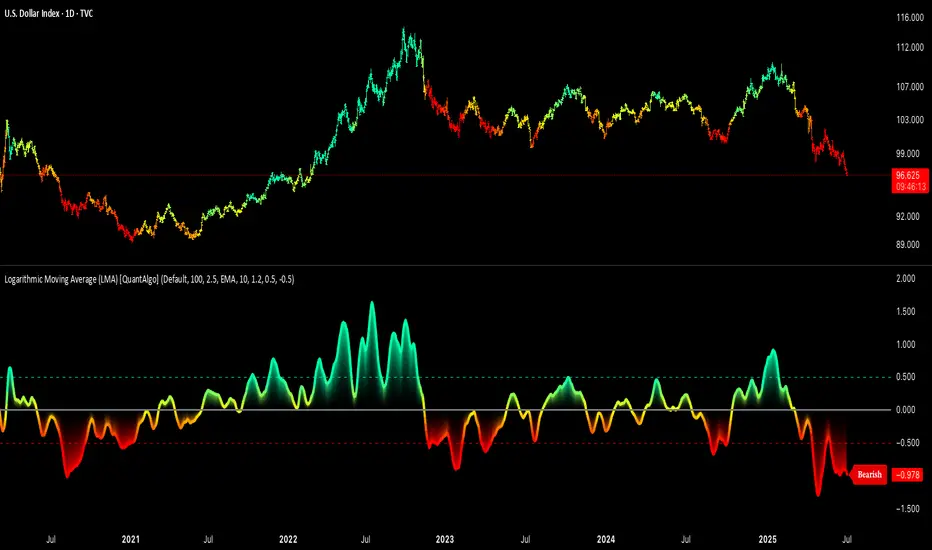
Volumatic Support/Resistance Levels [BigBeluga]🔵 OVERVIEW
A smart volume-powered tool for identifying key support and resistance zones—enhanced with real-time volume histogram fills and high-volume markers.
Volumatic Support/Resistance Levels detects structural levels from swing highs and lows, and wraps them in dynamic histograms that reflect the relative volume strength around those zones. It highlights the strongest price levels not just by structure—but by the weight of market participation.
🔵 CONCEPTS
Price Zones: Support and resistance levels are drawn from recent price pivots, while volume is used to visually enhance these zones with filled histograms and highlight moments of peak activity using markers.
Histogram Fill = Activity Zone: The width and intensity of each filled zone adjusts to recent volume bursts.
High-Volume Alerts: Circle markers highlight moments of volume dominance directly on the levels—revealing pressure points of support/resistance.
Clean Visual Encoding: Red = resistance zones, green = support zones, orange = high-volume bars.
🔵 FEATURES
Detects pivot-based resistance (highs) and support (lows) using a customizable range length.
Wraps these levels in volume-weighted bands that expand/contract based on percentile volume.
Color fill intensity increases with rising volume pressure, creating a live histogram feel.
When volume > user-defined threshold , the indicator adds circle markers at the top and bottom of that price level zone.
Bar coloring highlights the candles that generated this high-volume behavior (orange by default).
Adjustable settings for all thresholds and colors, so traders can dial in volume sensitivity.
🔵 HOW TO USE
Identify volume-confirmed resistance and support zones for potential reversal or breakout setups.
Focus on levels with intense histogram fill and circle markers —they indicate strong participation.
Use bar coloring to track when key activity started and align it with broader market context.
Works well in combination with order blocks, trend indicators, or liquidity zones.
Ideal for day traders, scalpers, and volume-sensitive setups.
🔵 CONCLUSION
Volumatic Support/Resistance Levels elevates traditional support and resistance logic by anchoring it in volume context. Instead of relying solely on price action, it gives traders insight into where real conviction lies—by mapping how aggressively the market defended or rejected key levels. It's a visual, reactive, and volume-conscious upgrade to your structural toolkit.

True Close – Institutional Trading Sessions (Zeiierman)█ Overview
True Close – Institutional Trading Sessions (Zeiierman) is a professional-grade session mapping tool designed to help traders align with how institutions perceive the market’s true close. Unlike the textbook “daily close” used by retail traders, institutional desks often anchor their risk management, execution benchmarks, and exposure metrics to the first hour of the next session.
This indicator visualizes that logic directly on your chart — drawing session boxes, true close levels, and time-aligned labels across Sydney, Tokyo, London, and New York. It highlights the first hour of each session, projects the institutional closing price, and builds a live dashboard that tells you which sessions are active, which are in the critical opening phase, and what levels matter most right now.
More than just a visual tool, this indicator embeds institutional rhythm directly into your workflow — giving you a window into where big players finalize yesterday’s business, rebalance exposure, and execute delayed orders. It’s not just about painting sessions on your chart — it’s about adopting the mindset of those who truly move the market. Institutions don’t settle risk at the bell; they complete it in the next session. This tool lets you see that transition in real time, giving you an edge that goes beyond candles and indicators.
█ How It Works
⚪ Session Detection Engine
Each session is identified by its own time block (e.g., 09:00–17:30 for London). Once a session opens:
A full-session box is drawn to track its range.
The first hour is highlighted separately.
Once the first hour completes, the true close line is plotted, representing the price institutions often treat as the "real" close of the prior day.
⚪ Institutional True Close Logic
The script captures the close of the first hour, not the end of the day.
This line becomes a static reference across your chart, letting you visualize how price interacts with that institutional anchor:
Rejections from it show where yesterday's flow is respected.
Breaks through it may indicate that today's flows are rewriting the narrative.
⚪ Dynamic Dashboard Table
A live table appears in the corner of your screen, showing:
Each session's active status
Whether we’re inside the first hour
The current “true close” price if available
Each cell comes with advanced tooltips giving institutional context, flow dynamics, and market microstructure insights — from rebalancing spillovers to VWAP/TWAP lag effects.
█ How to Use
⚪ Use the First-Hour Line as Your Institutional Anchor
Treat it like the price level that big funds care about. Watch how the price behaves around level. Fades, re-tests, or continuation moves often occur as the market finishes recapping yesterday’s leftover orders.
⚪ Structure Entries Around the Session Context
Are you inside the first hour? Expect more volatility, more decisive flow. After the first session hour, expect fading liquidity as the market slows down and awaits the next session to open.
█ Settings
UTC Offset – Select your preferred time zone; all sessions adjust accordingly.
Session Toggles – Enable/disable Sydney, Tokyo, London, or NY.
Box Display Options – Show/hide session background, first-hour fill, borders.
True Close Line Controls – Enable line, label, and customize width & color.
Execution Hour Labels – Optional toggle for first-hour label placement.
-----------------
Disclaimer
The content provided in my scripts, indicators, ideas, algorithms, and systems is for educational and informational purposes only. It does not constitute financial advice, investment recommendations, or a solicitation to buy or sell any financial instruments. I will not accept liability for any loss or damage, including without limitation any loss of profit, which may arise directly or indirectly from the use of or reliance on such information.
All investments involve risk, and the past performance of a security, industry, sector, market, financial product, trading strategy, backtest, or individual's trading does not guarantee future results or returns. Investors are fully responsible for any investment decisions they make. Such decisions should be based solely on an evaluation of their financial circumstances, investment objectives, risk tolerance, and liquidity needs.

Open Interest Footprint IQ [TradingIQ]Hello Traders!
Th e Open Interest Footprint IQ indicator is an advanced visualization tool designed for cryptocurrency markets. It provides a granular, real-time breakdown of open interest changes across different price levels, allowing traders to see how aggressive market participation is distributed within each bar.
Unlike standard footprint charts that rely solely on volume, this indicator offers unique insights by focusing on the interaction between price action and changes in open interest (OI) — a leading metric often used to infer trader intent and positioning.
How it works
The Open Interest Footprint IQ processes lower timeframe price and open interest data to build a footprint-style chart that shows how traders are positioning themselves within each candle.
Here’s a breakdown of the process:
1. Granular OI & Price Sampling
The script retrieves lower-timeframe data (1-minute, 1-second, or 1-tick, based on your setting).
For each candle, it captures:
High and low prices
Price change direction
Change in open interest (OI)
2. Classifying Trader Behavior
For each lower-timeframe segment, the indicator determines the type of positioning occurring based on price movement and OI change:
If price is moving up and open interest is increasing, it suggests that long positions are being opened. This is considered a "Longs Opening" event, labeled as UU (Up/Up).
If price is moving up but open interest is decreasing, it indicates that short positions are being closed. This is referred to as UD (Up/Down), or "Shorts Closing."
If price is moving down and open interest is increasing, it signals that short positions are being opened. This is known as DU (Down/Up), or "Shorts Opening."
If price is moving down while open interest is also decreasing, it means that long positions are being closed. This is labeled as DD (Down/Down), or "Longs Closing."
These are stored in separate arrays and displayed at specific price levels.
It is particularly useful for identifying:
Where longs or shorts are opening/closing positions
Stacked imbalances (indicative of potential absorption or exhaustion)
Value area zones and POC (Point of Control) based on OI, not volume
This footprint runs on your choice of sub-bar granularity and is ideal for high-frequency trading, scalping, and entries based on order flow dynamics.
Key Features
Footprint Visualization
At each price level within a candle:
Long/short opening and closing behavior is broken down.
Delta (net open interest change) is displayed both numerically and color-coded.
Optional gradient coloring shows intensity and type of flow (longs/shorts opened/closed).
Cumulative or per-bar reset modes allow you to track OI evolution over time.
The image above explains the information that each Footprint box shows across a candlestick!
Each footprint box shows:
OI Delta
OI Delta %
Longs Opened (LO)
Longs Closed (LC)
Shorts Opened (SO)
Shorts Closed (SC)
The image above explains the color-coding feature of the indicator.
Boxes are color coded to show which position action
dominated at the price area.
For this example:
Green boxes = Long positions being opened dominated
Purple boxes = Long positions being closed dominated
Red boxes = Short positions being opened dominated
Yellow boxes = Short positions being closed dominated
All colors are customizable.
Additionally, for traders who are only interested in whether OI increased/decreased, a "two-color" option is available in the settings.
For the two-color option, footprint boxes can be one of two colors. Showing whether OI increased or decreased at the level.
Cumulative Levels
Open Interest Footprint IQ contains a "Cumulative Levels" feature that tracks/stores open interest change at tick levels over time, rather than resetting per bar.
With the "Cumulative Levels" feature enabled, traders can see open interest changes persist across all candlesticks. This feature is useful for determining whether longs opening, longs closing, shorts opening, or shorts closing are dominating at particular price areas over time rather than on a single bar.
A useful feature to see if shorts/longs are favoring certain price throughout the day, week, month, etc.
Input Settings Explained
Granularity (Dropdown: Granularity)
Options: 1-Minute, 1-Second, 1-Tick
Determines how finely the script samples the lower timeframe data to construct the footprint.
For precision:
1-Tick = Highest accuracy, but more resource-intensive.
1-Second/1-Minute = Suitable for broader or more zoomed-out analysis.
Tick Level Distance (Tick Level Distance (0 = Auto))
Defines the vertical spacing between levels in the footprint chart.
If 0, the script uses an automatic calculation based on ATR to adapt to volatility.
Set a manual value (e.g., 5) to control the height granularity of each level in ticks.
Cumulative Levels (Toggle)
If enabled, the footprint builds cumulatively over time, rather than resetting per candle.
Use case: Visualize ongoing buildup of OI activity across a session or day.
Cumulative Levels Reset TF (Timeframe)
Sets the reset interval for the cumulative view (e.g., reset daily, hourly, etc.)
Works only when Cumulative Levels is enabled.
Delta Box Display Settings
Show Delta Percentage
Toggles the display of the percentage change in OI across the footprint level.
Helpful to gauge how aggressive positioning is relative to total OI at that level.
Show Longs/Shorts (Opened/Closed)
Show Longs Opened: Displays OI increase in up candles (price ↑, OI ↑).
Show Longs Closed: Displays OI decrease in down candles (price ↓, OI ↓).
Show Shorts Opened: OI increase in down candles (price ↓, OI ↑).
Show Shorts Closed: OI decrease in up candles (price ↑, OI ↓).
These behaviors are color-coded to give traders instant context:
Blue-green for longs opening.
Purple for longs closing.
Red for shorts opening.
Yellow for shorts closing.
Value Area & POC
Value Area % (Value Area %)
Controls how much cumulative open interest is used to define the value area.
Example: 70% means the smallest range of prices that contains 70% of total OI in that bar will be marked.
Helps identify zones of interest, support/resistance, and institutional levels.
The image above explains how to identify the VAH/VAL/POC shown by Open Interest Footprint IQ.
VAH = Upper 🞂
POC = ●
VAL = Lower 🞂
Imbalances
Imbalance Percentage
Defines the minimum delta % required at a level to be marked as an imbalance.
If the net open interest change at a level exceeds this threshold, a visual marker appears.
Stacked Imbalance Count
If the number of consecutive imbalance levels meets this count, a “Stacked Imbalance” alert will trigger.
This can signal aggressive buying or selling pressure, potential breakout zones, or institutional absorption.
Color Settings
Longs Opened / Closed, Shorts Opened / Closed
Customize the color palette for each order flow behavior.
These colors appear in the background gradient of the footprint boxes.
Up/Down Only Mode
Toggle to override all behavior-based colors with a single Up Color and Down Color.
Useful if you prefer a simple bull/bear view.
Up Color / Down Color
If "Up/Down Only" is enabled, these two colors are used to represent all net positive or negative deltas.
Special Notes
Crypto only: This script works only with crypto tickers on TradingView.
For other assets (stocks, futures), a warning message will appear instead.
OI data must be available from the exchange (many perpetual pairs support this).
If the footprint is too small or invisible, increase your tick level spacing in the settings.
Alerts
When a stacked imbalance is detected, an alert is fired ("Stacked Imbalance").
This feature is useful for automated systems, bots, or simply staying informed of potential trade setups.
And that's all for now!
If you have any questions or features you'd like to see feel free to share them in the comments below!
Thank you traders!
Zigzag CandlesCan't deny that I am obsessed with zigzags. Been doing some crazy experiments with it and have many more in pipeline. I believe zigzag can be used to derive better trend following methods. Here is an attempt to visualize zigzag as candlesticks. Next steps probably to derive moving average, atr (although there was an attempt of AZR made earlier) and probably supertrend too ;)
Input parameters include ZigzagLength (to calculate zigzag) and CandleSize (number of zigzag pivots in each candle)
CandleSize can be 3 or more. Every time we collect pivots which are equal to CandleSize, we derive one candle. And when we derive a candle, we remove all old pivots except the last one. Becauase, the last pivot acts as open to the next bar and is required.
Body of the candle tells the start and end zigzag pivot in the range. And Wicks signify highest and lowest pivots in the range. High and Low wicks are placed at the pivot where high and lows are formed. Hence, you can see them at different positions each time.
Thanks to @RicardoSantos for suggesting boxes for candles - while I was trying to achieve this with plotbar

MathStatisticsKernelFunctionsLibrary "MathStatisticsKernelFunctions"
TODO: add library description here
uniform(distance, bandwidth) Uniform kernel.
Parameters:
distance : float, distance to kernel origin.
bandwidth : float, default=1.0, bandwidth limiter to weight the kernel.
Returns: float.
triangular(distance, bandwidth) Triangular kernel.
Parameters:
distance : float, distance to kernel origin.
bandwidth : float, default=1.0, bandwidth limiter to weight the kernel.
Returns: float.
epanechnikov(distance, bandwidth) Epanechnikov kernel.
Parameters:
distance : float, distance to kernel origin.
bandwidth : float, default=1.0, bandwidth limiter to weight the kernel.
Returns: float.
quartic(distance, bandwidth) Quartic kernel.
Parameters:
distance : float, distance to kernel origin.
bandwidth : float, default=1.0, bandwidth limiter to weight the kernel.
Returns: float.
triweight(distance, bandwidth) Triweight kernel.
Parameters:
distance : float, distance to kernel origin.
bandwidth : float, default=1.0, bandwidth limiter to weight the kernel.
Returns: float.
tricubic(distance, bandwidth) Tricubic kernel.
Parameters:
distance : float, distance to kernel origin.
bandwidth : float, default=1.0, bandwidth limiter to weight the kernel.
Returns: float.
gaussian(distance, bandwidth) Gaussian kernel.
Parameters:
distance : float, distance to kernel origin.
bandwidth : float, default=1.0, bandwidth limiter to weight the kernel.
Returns: float.
cosine(distance, bandwidth) Cosine kernel.
Parameters:
distance : float, distance to kernel origin.
bandwidth : float, default=1.0, bandwidth limiter to weight the kernel.
Returns: float.
logistic(distance, bandwidth) logistic kernel.
Parameters:
distance : float, distance to kernel origin.
bandwidth : float, default=1.0, bandwidth limiter to weight the kernel.
Returns: float.
sigmoid(distance, bandwidth) Sigmoid kernel.
Parameters:
distance : float, distance to kernel origin.
bandwidth : float, default=1.0, bandwidth limiter to weight the kernel.
Returns: float.
select(kernel, distance, bandwidth) Kernel selection method.
Parameters:
kernel : string, kernel to select. (options="uniform", "triangle", "epanechnikov", "quartic", "triweight", "tricubic", "gaussian", "cosine", "logistic", "sigmoid")
distance : float, distance to kernel origin.
bandwidth : float, default=1.0, bandwidth limiter to weight the kernel.
Returns: float.
MathConstantsLibrary "MathConstants"
Mathematical Constants
E() The number e
Log2E() The number log (e)
Log10E() The number log (e)
Ln2() The number log (2)
Ln10() The number log (10)
LnPi() The number log (pi)
Ln2PiOver2() The number log (2*pi)/2
InvE() The number 1/e
SqrtE() The number sqrt(e)
Sqrt2() The number sqrt(2)
Sqrt3() The number sqrt(3)
Sqrt1Over2() The number sqrt(1/2) = 1/sqrt(2) = sqrt(2)/2
HalfSqrt3() The number sqrt(3)/2
Pi() The number pi
Pi2() The number pi*2
PiOver2() The number pi/2
Pi3Over2() The number pi*3/2
PiOver4() The number pi/4
SqrtPi() The number sqrt(pi)
Sqrt2Pi() The number sqrt(2pi)
SqrtPiOver2() The number sqrt(pi/2)
Sqrt2PiE() The number sqrt(2*pi*e)
LogSqrt2Pi() The number log(sqrt(2*pi))
LogSqrt2PiE() The number log(sqrt(2*pi*e))
LogTwoSqrtEOverPi() The number log(2 * sqrt(e / pi))
InvPi() The number 1/pi
TwoInvPi() The number 2/pi
InvSqrtPi() The number 1/sqrt(pi)
InvSqrt2Pi() The number 1/sqrt(2pi)
TwoInvSqrtPi() The number 2/sqrt(pi)
TwoSqrtEOverPi() The number 2 * sqrt(e / pi)
Degree() The number (pi)/180 - factor to convert from Degree (deg) to Radians (rad).
Grad() The number (pi)/200 - factor to convert from NewGrad (grad) to Radians (rad).
PowerDecibel() The number ln(10)/20 - factor to convert from Power Decibel (dB) to Neper (Np). Use this version when the Decibel represent a power gain but the compared values are not powers (e.g. amplitude, current, voltage).
NeutralDecibel() The number ln(10)/10 - factor to convert from Neutral Decibel (dB) to Neper (Np). Use this version when either both or neither of the Decibel and the compared values represent powers.
Catalan() The Catalan constant
Sum(k=0 -> inf){ (-1)^k/(2*k + 1)2 }
EulerMascheroni() The Euler-Mascheroni constant
lim(n -> inf){ Sum(k=1 -> n) { 1/k - log(n) } }
GoldenRatio() The number (1+sqrt(5))/2, also known as the golden ratio
Glaisher() The Glaisher constant
e^(1/12 - Zeta(-1))
Khinchin() The Khinchin constant
prod(k=1 -> inf){1+1/(k*(k+2))^log(k,2)}

taLibrary "ta"
█ OVERVIEW
This library holds technical analysis functions calculating values for which no Pine built-in exists.
Look first. Then leap.
█ FUNCTIONS
cagr(entryTime, entryPrice, exitTime, exitPrice)
It calculates the "Compound Annual Growth Rate" between two points in time. The CAGR is a notional, annualized growth rate that assumes all profits are reinvested. It only takes into account the prices of the two end points — not drawdowns, so it does not calculate risk. It can be used as a yardstick to compare the performance of two instruments. Because it annualizes values, the function requires a minimum of one day between the two end points (annualizing returns over smaller periods of times doesn't produce very meaningful figures).
Parameters:
entryTime : The starting timestamp.
entryPrice : The starting point's price.
exitTime : The ending timestamp.
exitPrice : The ending point's price.
Returns: CAGR in % (50 is 50%). Returns `na` if there is not >=1D between `entryTime` and `exitTime`, or until the two time points have not been reached by the script.
█ v2, Mar. 8, 2022
Added functions `allTimeHigh()` and `allTimeLow()` to find the highest or lowest value of a source from the first historical bar to the current bar. These functions will not look ahead; they will only return new highs/lows on the bar where they occur.
allTimeHigh(src)
Tracks the highest value of `src` from the first historical bar to the current bar.
Parameters:
src : (series int/float) Series to track. Optional. The default is `high`.
Returns: (float) The highest value tracked.
allTimeLow(src)
Tracks the lowest value of `src` from the first historical bar to the current bar.
Parameters:
src : (series int/float) Series to track. Optional. The default is `low`.
Returns: (float) The lowest value tracked.
█ v3, Sept. 27, 2022
This version includes the following new functions:
aroon(length)
Calculates the values of the Aroon indicator.
Parameters:
length (simple int) : (simple int) Number of bars (length).
Returns: ( [float, float ]) A tuple of the Aroon-Up and Aroon-Down values.
coppock(source, longLength, shortLength, smoothLength)
Calculates the value of the Coppock Curve indicator.
Parameters:
source (float) : (series int/float) Series of values to process.
longLength (simple int) : (simple int) Number of bars for the fast ROC value (length).
shortLength (simple int) : (simple int) Number of bars for the slow ROC value (length).
smoothLength (simple int) : (simple int) Number of bars for the weigted moving average value (length).
Returns: (float) The oscillator value.
dema(source, length)
Calculates the value of the Double Exponential Moving Average (DEMA).
Parameters:
source (float) : (series int/float) Series of values to process.
length (simple int) : (simple int) Length for the smoothing parameter calculation.
Returns: (float) The double exponentially weighted moving average of the `source`.
dema2(src, length)
An alternate Double Exponential Moving Average (Dema) function to `dema()`, which allows a "series float" length argument.
Parameters:
src : (series int/float) Series of values to process.
length : (series int/float) Length for the smoothing parameter calculation.
Returns: (float) The double exponentially weighted moving average of the `src`.
dm(length)
Calculates the value of the "Demarker" indicator.
Parameters:
length (simple int) : (simple int) Number of bars (length).
Returns: (float) The oscillator value.
donchian(length)
Calculates the values of a Donchian Channel using `high` and `low` over a given `length`.
Parameters:
length (int) : (series int) Number of bars (length).
Returns: ( [float, float, float ]) A tuple containing the channel high, low, and median, respectively.
ema2(src, length)
An alternate ema function to the `ta.ema()` built-in, which allows a "series float" length argument.
Parameters:
src : (series int/float) Series of values to process.
length : (series int/float) Number of bars (length).
Returns: (float) The exponentially weighted moving average of the `src`.
eom(length, div)
Calculates the value of the Ease of Movement indicator.
Parameters:
length (simple int) : (simple int) Number of bars (length).
div (simple int) : (simple int) Divisor used for normalzing values. Optional. The default is 10000.
Returns: (float) The oscillator value.
frama(source, length)
The Fractal Adaptive Moving Average (FRAMA), developed by John Ehlers, is an adaptive moving average that dynamically adjusts its lookback period based on fractal geometry.
Parameters:
source (float) : (series int/float) Series of values to process.
length (int) : (series int) Number of bars (length).
Returns: (float) The fractal adaptive moving average of the `source`.
ft(source, length)
Calculates the value of the Fisher Transform indicator.
Parameters:
source (float) : (series int/float) Series of values to process.
length (simple int) : (simple int) Number of bars (length).
Returns: (float) The oscillator value.
ht(source)
Calculates the value of the Hilbert Transform indicator.
Parameters:
source (float) : (series int/float) Series of values to process.
Returns: (float) The oscillator value.
ichimoku(conLength, baseLength, senkouLength)
Calculates values of the Ichimoku Cloud indicator, including tenkan, kijun, senkouSpan1, senkouSpan2, and chikou. NOTE: offsets forward or backward can be done using the `offset` argument in `plot()`.
Parameters:
conLength (int) : (series int) Length for the Conversion Line (Tenkan). The default is 9 periods, which returns the mid-point of the 9 period Donchian Channel.
baseLength (int) : (series int) Length for the Base Line (Kijun-sen). The default is 26 periods, which returns the mid-point of the 26 period Donchian Channel.
senkouLength (int) : (series int) Length for the Senkou Span 2 (Leading Span B). The default is 52 periods, which returns the mid-point of the 52 period Donchian Channel.
Returns: ( [float, float, float, float, float ]) A tuple of the Tenkan, Kijun, Senkou Span 1, Senkou Span 2, and Chikou Span values. NOTE: by default, the senkouSpan1 and senkouSpan2 should be plotted 26 periods in the future, and the Chikou Span plotted 26 days in the past.
ift(source)
Calculates the value of the Inverse Fisher Transform indicator.
Parameters:
source (float) : (series int/float) Series of values to process.
Returns: (float) The oscillator value.
kvo(fastLen, slowLen, trigLen)
Calculates the values of the Klinger Volume Oscillator.
Parameters:
fastLen (simple int) : (simple int) Length for the fast moving average smoothing parameter calculation.
slowLen (simple int) : (simple int) Length for the slow moving average smoothing parameter calculation.
trigLen (simple int) : (simple int) Length for the trigger moving average smoothing parameter calculation.
Returns: ( [float, float ]) A tuple of the KVO value, and the trigger value.
pzo(length)
Calculates the value of the Price Zone Oscillator.
Parameters:
length (simple int) : (simple int) Length for the smoothing parameter calculation.
Returns: (float) The oscillator value.
rms(source, length)
Calculates the Root Mean Square of the `source` over the `length`.
Parameters:
source (float) : (series int/float) Series of values to process.
length (int) : (series int) Number of bars (length).
Returns: (float) The RMS value.
rwi(length)
Calculates the values of the Random Walk Index.
Parameters:
length (simple int) : (simple int) Lookback and ATR smoothing parameter length.
Returns: ( [float, float ]) A tuple of the `rwiHigh` and `rwiLow` values.
stc(source, fast, slow, cycle, d1, d2)
Calculates the value of the Schaff Trend Cycle indicator.
Parameters:
source (float) : (series int/float) Series of values to process.
fast (simple int) : (simple int) Length for the MACD fast smoothing parameter calculation.
slow (simple int) : (simple int) Length for the MACD slow smoothing parameter calculation.
cycle (simple int) : (simple int) Number of bars for the Stochastic values (length).
d1 (simple int) : (simple int) Length for the initial %D smoothing parameter calculation.
d2 (simple int) : (simple int) Length for the final %D smoothing parameter calculation.
Returns: (float) The oscillator value.
stochFull(periodK, smoothK, periodD)
Calculates the %K and %D values of the Full Stochastic indicator.
Parameters:
periodK (simple int) : (simple int) Number of bars for Stochastic calculation. (length).
smoothK (simple int) : (simple int) Number of bars for smoothing of the %K value (length).
periodD (simple int) : (simple int) Number of bars for smoothing of the %D value (length).
Returns: ( [float, float ]) A tuple of the slow %K and the %D moving average values.
stochRsi(lengthRsi, periodK, smoothK, periodD, source)
Calculates the %K and %D values of the Stochastic RSI indicator.
Parameters:
lengthRsi (simple int) : (simple int) Length for the RSI smoothing parameter calculation.
periodK (simple int) : (simple int) Number of bars for Stochastic calculation. (length).
smoothK (simple int) : (simple int) Number of bars for smoothing of the %K value (length).
periodD (simple int) : (simple int) Number of bars for smoothing of the %D value (length).
source (float) : (series int/float) Series of values to process. Optional. The default is `close`.
Returns: ( [float, float ]) A tuple of the slow %K and the %D moving average values.
supertrend(factor, atrLength, wicks)
Calculates the values of the SuperTrend indicator with the ability to take candle wicks into account, rather than only the closing price.
Parameters:
factor (float) : (series int/float) Multiplier for the ATR value.
atrLength (simple int) : (simple int) Length for the ATR smoothing parameter calculation.
wicks (simple bool) : (simple bool) Condition to determine whether to take candle wicks into account when reversing trend, or to use the close price. Optional. Default is false.
Returns: ( [float, int ]) A tuple of the superTrend value and trend direction.
szo(source, length)
Calculates the value of the Sentiment Zone Oscillator.
Parameters:
source (float) : (series int/float) Series of values to process.
length (simple int) : (simple int) Length for the smoothing parameter calculation.
Returns: (float) The oscillator value.
t3(source, length, vf)
Calculates the value of the Tilson Moving Average (T3).
Parameters:
source (float) : (series int/float) Series of values to process.
length (simple int) : (simple int) Length for the smoothing parameter calculation.
vf (simple float) : (simple float) Volume factor. Affects the responsiveness.
Returns: (float) The Tilson moving average of the `source`.
t3Alt(source, length, vf)
An alternate Tilson Moving Average (T3) function to `t3()`, which allows a "series float" `length` argument.
Parameters:
source (float) : (series int/float) Series of values to process.
length (float) : (series int/float) Length for the smoothing parameter calculation.
vf (simple float) : (simple float) Volume factor. Affects the responsiveness.
Returns: (float) The Tilson moving average of the `source`.
tema(source, length)
Calculates the value of the Triple Exponential Moving Average (TEMA).
Parameters:
source (float) : (series int/float) Series of values to process.
length (simple int) : (simple int) Length for the smoothing parameter calculation.
Returns: (float) The triple exponentially weighted moving average of the `source`.
tema2(source, length)
An alternate Triple Exponential Moving Average (TEMA) function to `tema()`, which allows a "series float" `length` argument.
Parameters:
source (float) : (series int/float) Series of values to process.
length (float) : (series int/float) Length for the smoothing parameter calculation.
Returns: (float) The triple exponentially weighted moving average of the `source`.
trima(source, length)
Calculates the value of the Triangular Moving Average (TRIMA).
Parameters:
source (float) : (series int/float) Series of values to process.
length (int) : (series int) Number of bars (length).
Returns: (float) The triangular moving average of the `source`.
trima2(src, length)
An alternate Triangular Moving Average (TRIMA) function to `trima()`, which allows a "series int" length argument.
Parameters:
src : (series int/float) Series of values to process.
length : (series int) Number of bars (length).
Returns: (float) The triangular moving average of the `src`.
trix(source, length, signalLength, exponential)
Calculates the values of the TRIX indicator.
Parameters:
source (float) : (series int/float) Series of values to process.
length (simple int) : (simple int) Length for the smoothing parameter calculation.
signalLength (simple int) : (simple int) Length for smoothing the signal line.
exponential (simple bool) : (simple bool) Condition to determine whether exponential or simple smoothing is used. Optional. The default is `true` (exponential smoothing).
Returns: ( [float, float, float ]) A tuple of the TRIX value, the signal value, and the histogram.
uo(fastLen, midLen, slowLen)
Calculates the value of the Ultimate Oscillator.
Parameters:
fastLen (simple int) : (series int) Number of bars for the fast smoothing average (length).
midLen (simple int) : (series int) Number of bars for the middle smoothing average (length).
slowLen (simple int) : (series int) Number of bars for the slow smoothing average (length).
Returns: (float) The oscillator value.
vhf(source, length)
Calculates the value of the Vertical Horizontal Filter.
Parameters:
source (float) : (series int/float) Series of values to process.
length (simple int) : (simple int) Number of bars (length).
Returns: (float) The oscillator value.
vi(length)
Calculates the values of the Vortex Indicator.
Parameters:
length (simple int) : (simple int) Number of bars (length).
Returns: ( [float, float ]) A tuple of the viPlus and viMinus values.
vzo(length)
Calculates the value of the Volume Zone Oscillator.
Parameters:
length (simple int) : (simple int) Length for the smoothing parameter calculation.
Returns: (float) The oscillator value.
williamsFractal(period)
Detects Williams Fractals.
Parameters:
period (int) : (series int) Number of bars (length).
Returns: ( [bool, bool ]) A tuple of an up fractal and down fractal. Variables are true when detected.
wpo(length)
Calculates the value of the Wave Period Oscillator.
Parameters:
length (simple int) : (simple int) Length for the smoothing parameter calculation.
Returns: (float) The oscillator value.
█ v7, Nov. 2, 2023
This version includes the following new and updated functions:
atr2(length)
An alternate ATR function to the `ta.atr()` built-in, which allows a "series float" `length` argument.
Parameters:
length (float) : (series int/float) Length for the smoothing parameter calculation.
Returns: (float) The ATR value.
changePercent(newValue, oldValue)
Calculates the percentage difference between two distinct values.
Parameters:
newValue (float) : (series int/float) The current value.
oldValue (float) : (series int/float) The previous value.
Returns: (float) The percentage change from the `oldValue` to the `newValue`.
donchian(length)
Calculates the values of a Donchian Channel using `high` and `low` over a given `length`.
Parameters:
length (int) : (series int) Number of bars (length).
Returns: ( [float, float, float ]) A tuple containing the channel high, low, and median, respectively.
highestSince(cond, source)
Tracks the highest value of a series since the last occurrence of a condition.
Parameters:
cond (bool) : (series bool) A condition which, when `true`, resets the tracking of the highest `source`.
source (float) : (series int/float) Series of values to process. Optional. The default is `high`.
Returns: (float) The highest `source` value since the last time the `cond` was `true`.
lowestSince(cond, source)
Tracks the lowest value of a series since the last occurrence of a condition.
Parameters:
cond (bool) : (series bool) A condition which, when `true`, resets the tracking of the lowest `source`.
source (float) : (series int/float) Series of values to process. Optional. The default is `low`.
Returns: (float) The lowest `source` value since the last time the `cond` was `true`.
relativeVolume(length, anchorTimeframe, isCumulative, adjustRealtime)
Calculates the volume since the last change in the time value from the `anchorTimeframe`, the historical average volume using bars from past periods that have the same relative time offset as the current bar from the start of its period, and the ratio of these volumes. The volume values are cumulative by default, but can be adjusted to non-accumulated with the `isCumulative` parameter.
Parameters:
length (simple int) : (simple int) The number of periods to use for the historical average calculation.
anchorTimeframe (simple string) : (simple string) The anchor timeframe used in the calculation. Optional. Default is "D".
isCumulative (simple bool) : (simple bool) If `true`, the volume values will be accumulated since the start of the last `anchorTimeframe`. If `false`, values will be used without accumulation. Optional. The default is `true`.
adjustRealtime (simple bool) : (simple bool) If `true`, estimates the cumulative value on unclosed bars based on the data since the last `anchor` condition. Optional. The default is `false`.
Returns: ( [float, float, float ]) A tuple of three float values. The first element is the current volume. The second is the average of volumes at equivalent time offsets from past anchors over the specified number of periods. The third is the ratio of the current volume to the historical average volume.
rma2(source, length)
An alternate RMA function to the `ta.rma()` built-in, which allows a "series float" `length` argument.
Parameters:
source (float) : (series int/float) Series of values to process.
length (float) : (series int/float) Length for the smoothing parameter calculation.
Returns: (float) The rolling moving average of the `source`.
supertrend2(factor, atrLength, wicks)
An alternate SuperTrend function to `supertrend()`, which allows a "series float" `atrLength` argument.
Parameters:
factor (float) : (series int/float) Multiplier for the ATR value.
atrLength (float) : (series int/float) Length for the ATR smoothing parameter calculation.
wicks (simple bool) : (simple bool) Condition to determine whether to take candle wicks into account when reversing trend, or to use the close price. Optional. Default is `false`.
Returns: ( [float, int ]) A tuple of the superTrend value and trend direction.
vStop(source, atrLength, atrFactor)
Calculates an ATR-based stop value that trails behind the `source`. Can serve as a possible stop-loss guide and trend identifier.
Parameters:
source (float) : (series int/float) Series of values that the stop trails behind.
atrLength (simple int) : (simple int) Length for the ATR smoothing parameter calculation.
atrFactor (float) : (series int/float) The multiplier of the ATR value. Affects the maximum distance between the stop and the `source` value. A value of 1 means the maximum distance is 100% of the ATR value. Optional. The default is 1.
Returns: ( [float, bool ]) A tuple of the volatility stop value and the trend direction as a "bool".
vStop2(source, atrLength, atrFactor)
An alternate Volatility Stop function to `vStop()`, which allows a "series float" `atrLength` argument.
Parameters:
source (float) : (series int/float) Series of values that the stop trails behind.
atrLength (float) : (series int/float) Length for the ATR smoothing parameter calculation.
atrFactor (float) : (series int/float) The multiplier of the ATR value. Affects the maximum distance between the stop and the `source` value. A value of 1 means the maximum distance is 100% of the ATR value. Optional. The default is 1.
Returns: ( [float, bool ]) A tuple of the volatility stop value and the trend direction as a "bool".
Removed Functions:
allTimeHigh(src)
Tracks the highest value of `src` from the first historical bar to the current bar.
allTimeLow(src)
Tracks the lowest value of `src` from the first historical bar to the current bar.
trima2(src, length)
An alternate Triangular Moving Average (TRIMA) function to `trima()`, which allows a
"series int" length argument.
