Machine Learning Adaptive SuperTrend [AlgoAlpha]📈🤖 Machine Learning Adaptive SuperTrend - Take Your Trading to the Next Level! 🚀✨
Introducing the Machine Learning Adaptive SuperTrend , an advanced trading indicator designed to adapt to market volatility dynamically using machine learning techniques. This indicator employs k-means clustering to categorize market volatility into high, medium, and low levels, enhancing the traditional SuperTrend strategy. Perfect for traders who want an edge in identifying trend shifts and market conditions.
What is K-Means Clustering and How It Works
K-means clustering is a machine learning algorithm that partitions data into distinct groups based on similarity. In this indicator, the algorithm analyzes ATR (Average True Range) values to classify volatility into three clusters: high, medium, and low. The algorithm iterates to optimize the centroids of these clusters, ensuring accurate volatility classification.
Key Features
🎨 Customizable Appearance: Adjust colors for bullish and bearish trends.
🔧 Flexible Settings: Configure ATR length, SuperTrend factor, and initial volatility guesses.
📊 Volatility Classification: Uses k-means clustering to adapt to market conditions.
📈 Dynamic SuperTrend Calculation: Applies the classified volatility level to the SuperTrend calculation.
🔔 Alerts: Set alerts for trend shifts and volatility changes.
📋 Data Table Display: View cluster details and current volatility on the chart.
Quick Guide to Using the Machine Learning Adaptive SuperTrend Indicator
🛠 Add the Indicator: Add the indicator to favorites by pressing the star icon. Customize settings like ATR length, SuperTrend factor, and volatility percentiles to fit your trading style.
📊 Market Analysis: Observe the color changes and SuperTrend line for trend reversals. Use the data table to monitor volatility clusters.
🔔 Alerts: Enable notifications for trend shifts and volatility changes to seize trading opportunities without constant chart monitoring.
How It Works
The indicator begins by calculating the ATR values over a specified training period to assess market volatility. Initial guesses for high, medium, and low volatility percentiles are inputted. The k-means clustering algorithm then iterates to classify the ATR values into three clusters. This classification helps in determining the appropriate volatility level to apply to the SuperTrend calculation. As the market evolves, the indicator dynamically adjusts, providing real-time trend and volatility insights. The indicator also incorporates a data table displaying cluster centroids, sizes, and the current volatility level, aiding traders in making informed decisions.
Add the Machine Learning Adaptive SuperTrend to your TradingView charts today and experience a smarter way to trade! 🌟📊
Indicators and strategies

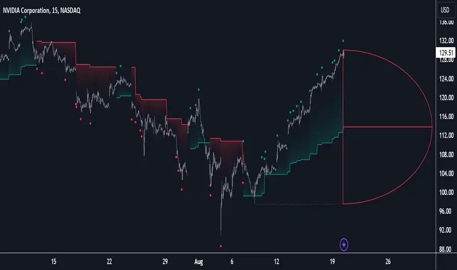
D-Shape Breakout Signals [LuxAlgo]The D-Shape Breakout Signals indicator uses a unique and novel technique to provide support/resistance curves, a trailing stop loss line, and visual breakout signals from semi-circular shapes.
🔶 USAGE
D-shape is a new concept where the distance between two Swing points is used to create a semi-circle/arc, where the width is expressed as a user-defined percentage of the radius. The resulting arc can be used as a potential support/resistance as well as a source of breakouts.
Users can adjust this percentage (width of the D-shape) in the settings ( "D-Width" ), which will influence breakouts and the Stop-Loss line.
🔹 Breakouts of D-Shape
The arc of this D-shape is used for detecting breakout signals between the price and the curve. Only one breakout per D-shape can occur.
A breakout is highlighted with a colored dot, signifying its location, with a green dot being used when the top part of the arc is exceeded, and red when the bottom part of the arc is surpassed.
When the price reaches the right side of the arc without breaking the arc top/bottom, a blue-colored dot is highlighted, signaling a "Neutral Breakout".
🔹 Trailing Stop-Loss Line
The script includes a Trailing Stop-Loss line (TSL), which is only updated when a breakout of the D-Shape occurs. The TSL will return the midline of the D-Shape subject to a breakout.
The TSL can be used as a stop-loss or entry-level but can also act as a potential support/resistance level or trend visualization.
🔶 DETAILS
A D-shape will initially be colored green when a Swing Low is followed by a Swing High, and red when a Swing Low is followed by a Swing High.
A breakout of the upper side of the D-shape will always update the color to green or to red when the breakout occurs in the lower part. A Neutral Breakout will result in a blue-colored D-shape. The transparency is lowered in the event of a breakout.
In the event of a D-shape breakout, the shape will be removed when the total number of visible D-Shapes exceeds the user set "Minimum Patterns" setting. Any D-shape whose boundaries have not been exceeded (and therefore still active) will remain visible.
🔹 Trailing Stop-Loss Line
Only when a breakout occurs will the midline of the D-shape closest to the closing price potentially become the new Trailing Stop value.
The script will only consider middle lines below the closing price on an upward breakout or middle lines above the closing price when it concerns a downward breakout.
In an uptrend, with an already available green TSL, the potential new Stop-Loss value must be higher than the previous TSL value; while in a downtrend, the new TSL value must be lower.
The Stop-Loss line won't be updated when a "Neutral Breakout" occurs.
🔶 SETTINGS
Swing Length: Period used for the swing detection, with higher values returning longer-term Swing Levels.
🔹 D-Patterns
Minimum Patterns: Minimum amount of visible D-Shape patterns.
D-Width: Width of the D-Shape as a percentage of the distance between both Swing Points.
Included Swings: Include "Swing High" (followed by a Swing Low), "Swing Low" (followed by a Swing High), or "Both"
Style Historical Patterns: Show the "Arc", "Midline" or "Both" of historical patterns.
🔹 Style
Label Size/Colors
Connecting Swing Level: Shows a line connecting the first Swing Point.
Color Fill: colorfill of Trailing Stop-Loss
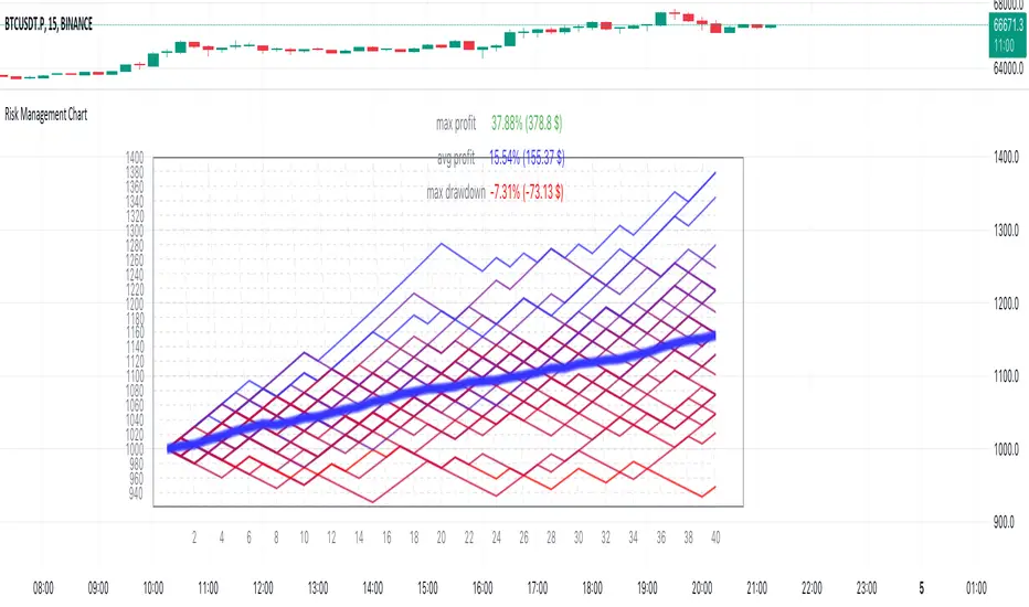
Monte Carlo (Polyline Traceback) [Kioseff Trading]Hello!
This script "Monte Carlo (Polyline Traceback) " performs a Monte Carlo simulation using polylines!
By using polylines, and tracing back the initial simulation to its origin point, we can better replicate the ideal output of a Monte Carlo simulation!
Such as:
The image above shows the output of a simulation (image sourced outside TV).
With this script, and polyline capabilities, we can come quite close on TradingView.
The image above shows the indicator in action! Not bad considering the ideal output.
Of course, the script is quite heavy and tries its best to circumvent limitations :D
You might run into load time errors, in which case you might try applying the built-in setting "Force Script Load". This setting will cut-off the visuals for some simulations, but has a higher chance of passing load-time limitations!
As shown in the image above, you can select to only show worst-case and best-case simulations. Using this option will reduce chart lag and improve load times.
Features
Monte Carlo Simulation: Performs Monte Carlo simulation to generate multiple future paths.
Asset Price: Can simulate future asset prices based on historical log returns.
Statistical Methods: Offers two simulation methods—Gaussian (Normal) distribution and Bootstrapping.
Adjustable Parameters: Offers numerous user-adjustable settings like number of simulations, forecast length, and more.
Historical Data Points: Option to specify the amount of historical data to be used in the simulation (price).
Best/Worst Case: Allows you to show only the best case / worst case outcome (range) for all simulations!
Thank you!

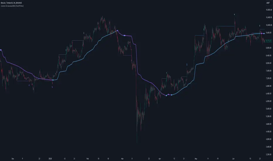
LOWESS (Locally Weighted Scatterplot Smoothing) [ChartPrime]LOWESS (Locally Weighted Scatterplot Smoothing)
⯁ OVERVIEW
The LOWESS (Locally Weighted Scatterplot Smoothing) [ ChartPrime ] indicator is an advanced technical analysis tool that combines LOWESS smoothing with a Modified Adaptive Gaussian Moving Average. This indicator provides traders with a sophisticated method for trend analysis, pivot point identification, and breakout detection.
◆ KEY FEATURES
LOWESS Smoothing: Implements Locally Weighted Scatterplot Smoothing for trend analysis.
Modified Adaptive Gaussian Moving Average: Incorporates a volatility-adapted Gaussian MA for enhanced trend detection.
Pivot Point Identification: Detects and visualizes significant pivot highs and lows.
Breakout Detection: Tracks and optionally displays the count of consecutive breakouts.
Gaussian Scatterplot: Offers a unique visualization of price movements using randomly colored points.
Customizable Parameters: Allows users to adjust calculation length, pivot detection, and visualization options.
◆ FUNCTIONALITY DETAILS
⬥ LOWESS Calculation:
Utilizes a weighted local regression to smooth price data.
Adapts to local trends, reducing noise while preserving important price movements.
⬥ Modified Adaptive Gaussian Moving Average:
Combines Gaussian weighting with volatility adaptation using ATR and standard deviation.
Smooths the Gaussian MA using LOWESS for enhanced trend visualization.
⬥ Pivot Point Detection and Visualization:
Identifies pivot highs and lows using customizable left and right bar counts.
Draws lines and labels to mark broke pivot points on the chart.
⬥ Breakout Tracking:
Monitors price crossovers of pivot lines to detect breakouts.
Optionally displays and updates the count of consecutive breakouts.
◆ USAGE
Trend Analysis: Use the color and direction of the smoothed Gaussian MA line to identify overall trend direction.
Breakout Trading: Monitor breakouts from pivot levels and their persistence using the breakout count feature.
Volatility Assessment: The spread of the Gaussian scatterplot can provide insights into market volatility.
⯁ USER INPUTS
Length: Sets the lookback period for LOWESS and Gaussian MA calculations (default: 30).
Pivot Length: Determines the number of bars to the left for pivot calculation (default: 5).
Count Breaks: Toggle to show the count of consecutive breakouts (default: false).
Gaussian Scatterplot: Toggle to display the Gaussian MA as a scatterplot (default: true).
⯁ TECHNICAL NOTES
Implements a custom LOWESS function for efficient local regression smoothing.
Uses a modified Gaussian MA calculation that adapts to market volatility.
Employs Pine Script's line and label drawing capabilities for clear pivot point visualization.
Utilizes random color generation for the Gaussian scatterplot to enhance visual distinction between different time periods.
The LOWESS (Locally Weighted Scatterplot Smoothing) indicator offers traders a sophisticated tool for trend analysis and breakout detection. By combining advanced smoothing techniques with pivot point analysis, it provides a comprehensive view of market dynamics. The indicator's adaptability to different market conditions and its customizable nature make it suitable for various trading styles and timeframes.
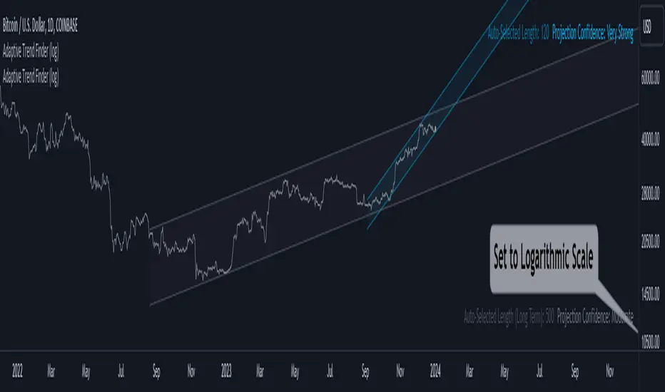
Adaptive Trend Finder (log)In the dynamic landscape of financial markets, the Adaptive Trend Finder (log) stands out as an example of precision and professionalism. This advanced tool, equipped with a unique feature, offers traders a sophisticated approach to market trend analysis: the choice between automatic detection of the long-term or short-term trend channel.
Key Features:
1. Choice Between Long-Term or Short-Term Trend Channel Detection: Positioned first, this distinctive feature of the Adaptive Trend Finder (log) allows traders to customize their analysis by choosing between the automatic detection of the long-term or short-term trend channel. This increased flexibility adapts to individual trading preferences and changing market conditions.
2. Autonomous Trend Channel Detection: Leveraging the robust statistical measure of the Pearson coefficient, the Adaptive Trend Finder (log) excels in autonomously locating the optimal trend channel. This data-driven approach ensures objective trend analysis, reducing subjective biases, and enhancing overall precision.
3. Precision of Logarithmic Scale: A distinctive characteristic of our indicator is its strategic use of the logarithmic scale for regression channels. This approach enables nuanced analysis of linear regression channels, capturing the subtleties of trends while accommodating variations in the amplitude of price movements.
4. Length and Strength Visualization: Traders gain a comprehensive view of the selected trend channel, with the revelation of its length and quantification of trend strength. These dual pieces of information empower traders to make informed decisions, providing insights into both the direction and intensity of the prevailing trend.
In the demanding universe of financial markets, the Adaptive Trend Finder (log) asserts itself as an essential tool for traders, offering an unparalleled combination of precision, professionalism, and customization. Highlighting the choice between automatic detection of the long-term or short-term trend channel in the first position, this indicator uniquely caters to the specific needs of each trader, ensuring informed decision-making in an ever-evolving financial environment.
Oscillator Scatterplot Analysis [Trendoscope®]In this indicator, we demonstrate how to plot oscillator behavior of oversold-overbought against price movements in the form of scatterplots and perform analysis. Scatterplots are drawn on a graph containing x and y-axis, where x represent one measure whereas y represents another. We use the library Graph to collect the data and plot it as scatterplot.
Pictorial explanation of components is defined in the chart below.
🎲 This indicator performs following tasks
Calculate and plot oscillator
Identify oversold and overbought areas based on various methods
Measure the price and bar movement from overbought to oversold and vice versa and plot them on the chart.
In our example,
The x-axis represents price movement. The plots found on the right side of the graph has positive price movements, whereas the plots found on the left side of the graph has negative price movements.
The y-axis represents the number of bars it took for reaching overbought to oversold and/or oversold to overbought. Positive bars mean we are measuring oversold to overbought, whereas negative bars are a measure of overbought to oversold.
🎲 Graph is divided into 4 equal quadrants
Quadrant 1 is the top right portion of the graph. Plots in this quadrant represent the instances where positive price movement is observed when the oscillator moved from oversold to overbought
Quadrant 2 is the top left portion of the graph. Plots in this quadrant represent the instances where negative price movement is observed when the oscillator moved from oversold to overbought.
Quadrant 3 is the bottom left portion of the chart. Plots in this quadrant represent the instances where negative price movement is observed when the oscillator moved from overbought to oversold.
Quadrant 4 is the bottom right portion of the chart. Plots in this quadrant represent the instances where positive price movement is observed when the oscillator moved from overbought to oversold.
🎲 Indicator components in Detail
Let's dive deep into the indicator.
🎯 Oscillator Selection
Select the Oscillator and define the overbought oversold conditions through input settings
Indicator - Oscillator base used for performing analysis
Length - Loopback length on which the oscillator is calculated
OB/OS Method - We use Bollinger Bands, Keltener Channel and Donchian channel to calculate dynamic overbought and oversold levels instead of static 80-10. This is also useful as other type of indicators may not be within 0-100 range.
Length and Multiplier are used for the bands for calculating Overbought/Oversold boundaries.
🎯 Define Graph Properties
Select different graph properties from the input settings that will instruct how to display the scatterplot.
Type - this can be either scatterplot or heatmap. Scatterplot will display plots with specific transparency to indicate the data, whereas heatmap will display background with different transparencies.
Plot Color - this is the color in which the scatterplot or heatmap is drawn
Plot Size - applicable mainly for scatterplot. Since the character we use for scatterplot is very tiny, the large at present looks optimal. But, based on the user's screen size, we may need to select different sizes so that it will render properly.
Rows and Columns - Number of rows and columns allocated per quadrant. This means, the total size of the chart is 2X rows and 2X columns. Data sets are divided into buckets based on the number of available rows and columns. Hence, changing this can change the appearance of the overall chart, even though they are representing the same data. Also, please note that tables can have max 10000 cells. If we increase the rows and columns by too much, we may get runtime errors.
Outliers - this is used to exclude the extreme data. 20% outlier means, the chart will ignore bottom 20% and top 20% when defining the chart boundaries. However, the extreme data is still added to the boundaries.

[Pandora] Vast Volatility Treasure TroveINTRODUCTION:
Volatility enthusiasts, prepare for VICTORY on this day of July 4th, 2024! This is my "Vast Volatility Treasure Trove," intended mostly for educational purposes, yet these functions will also exhibit versatility when combined with other algorithms to garner statistical excellence. Once again, I am now ripping the lid off of Pandora's box... of volatility. Inside this script is a 'vast' collection of volatility estimators, reflecting the indicators name. Whether you are a seasoned trader destined to navigate financial strife or an eagerly curious learner, this script offers a comprehensive toolkit for a broad spectrum of volatility analysis. Enjoy your journey through the realm of market volatility with this code!
WHAT IS MARKET VOLATILITY?:
Market volatility refers to various fluctuations in the value of a financial market or asset over a period of time, often characterized by occasional rapid and significant deviations in price. During periods of greater market volatility, evolving conditions of prices can move rapidly in either direction, creating uncertainty for investors with results of sharp declines as well as rapid gains. However, market volatility is a typical aspect expected in financial markets that can also present opportunities for informed decision-making and potential benefits from the price flux.
SCRIPT INTENTION:
Volatility is assuredly omnipresent, waxing and waning in magnitude, and some readers have every intention of studying and/or measuring it. This script serves as an all-in-one armada of volatility estimators for TradingView members. I set out to provide a diverse set of tools to analyze and interpret market volatility, offering volatile insights, and aid with the development of robust trading indicators and strategies.
In today's fast-paced financial markets, understanding and quantifying volatility is informative for both seasoned traders and novice investors. This script is designed to empower users by equipping them with a comprehensive suite of volatility estimators. Each function within this script has been meticulously crafted to address various aspects of volatility, from traditional methods like Garman-Klass and Parkinson to more advanced techniques like Yang-Zhang and my custom experimental algorithms.
Ultimately, this script is more than just a collection of functions. It is a gateway to a deeper understanding of market volatility and a valuable resource for anyone committed to mastering the complexities of financial markets.
SCRIPT CONTENTS:
This script includes a variety of functions designed to measure and analyze market volatility. Where applicable, an input checkbox option provides an unbiased/biased estimate. Below is a brief description of each function in the original order they appear as code upon first publish:
Parkinson Volatility - Estimates volatility emphasizing the high and low range movements.
Alternate Parkinson Volatility - Simpler version of the original Parkinson Volatility that I realized.
Garman-Klass Volatility - Estimates volatility based on high, low, open, and close prices using a formula that adjusts for biases in price dynamics.
Rogers-Satchell-Yoon Volatility #1 - Estimates volatility based on logarithmic differences between high, low, open, and close values.
Rogers-Satchell-Yoon Volatility #2 - Similar estimate to Rogers-Satchell with the same result via an alternate formulation of volatility.
Yang-Zhang Volatility - An advanced volatility estimate combining both strengths of the Garman-Klass and Rogers-Satchell estimators, with weights determined by an alpha parameter.
Yang-Zhang (Modified) Volatility - My experimental modification slightly different from the Yang-Zhang formula with improved computational efficiency.
Selectable Volatility - Basic customizable volatility calculation based on the logarithmic difference between selected numerator and denominator prices (e.g., open, high, low, close).
Close-to-Close Volatility - Estimates volatility using the logarithmic difference between consecutive closing prices. Specifically applicable to data sources without open, high, and low prices.
Open-to-Close Volatility - (Overnight Volatility): Estimates volatility based on the logarithmic difference between the opening price and the last closing price emphasizing overnight gaps.
Hilo Volatility - Estimates volatility using a method similar to Parkinson's method, which considers the logarithm of the high and low prices.
Vantage Volatility - My experimental custom 'vantage' method to estimate volatility similar to Yang-Zhang, which incorporates various factors (Alpha, Beta, Gamma) to generate a weighted logarithmic calculation. This may be a volatility advantage or disadvantage, hence it's name.
Schwert Volatility - Estimates volatility based on arithmetic returns.
Historical Volatility - Estimates volatility considering logarithmic returns.
Annualized Historical Volatility - Estimates annualized volatility using logarithmic returns, adjusted for the number of trading days in a year.
If I omitted any other known varieties, detailed requests for future consideration can be made below for their inclusion into this script within future versions...
BONUS ALGORITHMS:
This script also includes several experimental and bonus functions that push the boundaries of volatility analysis as I understand it. These functions are designed to provide additional insights and also are my ideal notions for traders looking to explore other methods of volatility measurement.
VOLATILITY APPLICATIONS:
Volatility estimators serve a common role across various facets of trading and financial analysis, offering insights into market behavior. These tools are already in instrumental with enhancing risk management practices by providing a deeper understanding of market dynamics and the inherent uncertainty in asset prices. With volatility estimators, traders can effectively quantifying market risk and adjust their strategies accordingly, optimizing portfolio performance and mitigating potential losses. Additionally, volatility estimations may serve as indication for detecting overbought or oversold market conditions, offering probabilistic insights that could inform strategic decisions at turning points. This script
distinctly offers a variety of volatility estimators to navigate intricate financial terrains with informed judgment to address challenges of strategic planning.
CODE REUSE:
You don't have to ask for my permission to use/reuse these functions in your published scripts, simply because I have better things to do than answer requests for the reuse of these functions.
Notice: Unfortunately, I will not provide any integration support into member's projects at all. I have my own projects that require way too much of my day already.

Linear Regression Oscillator [ChartPrime]Linear Regression Oscillator Indicator
Overview:
The Linear Regression Oscillator is a custom TradingView indicator designed to provide insights into potential mean reversion and trend conditions. By calculating a linear regression on the closing prices over a user-defined period, this oscillator helps identify overbought and oversold levels and highlights trend changes. The indicator also offers visual cues and color-coded price bars to aid in quick decision-making.
Key Features:
◆ Customizable Look-Back Period:
Input: Length
Default: 20
Description: Determines the period over which the linear regression is calculated. A longer period smooths the oscillator but may lag, while a shorter period is more responsive but may be noisier.
◆ Overbought and Oversold Thresholds:
Inputs: Upper Threshold and Lower Threshold
Default: 1.5 and -1.5 respectively
Description: Define the upper and lower bounds for identifying overbought and oversold conditions. Values outside these thresholds suggest potential reversals.
◆ Candlestick Color Plotting:
Input: Plot Bar Color
Default: false
Description: Option to color the price bars based on the oscillator's value, providing a visual representation of market conditions. Bars turn cyan for positive oscillator values and blue for negative.
◆ Mean Reversion and Trend Signals:
Visual markers and labels indicate when the oscillator suggests mean reversion or trend changes, aiding in identifying key market turning points.
◆ Invalidation Levels:
Tracks the highest and lowest prices over a recent period to set levels where the current trend signal would be considered invalidated.
◆ Gradient Color Coding:
Utilizes gradient color coding to enhance the visualization of oscillator values, making it easier to interpret overbought and oversold conditions.
◆ Usage Notes:
Setting the Look-Back Period:
Adjust the "Length" input based on the timeframe and the type of trading you are conducting. Shorter periods are more suited for intraday trading, while longer periods can be used for swing trading.
Interpreting Thresholds:
Use the upper and lower threshold inputs to fine-tune the sensitivity of the overbought and oversold signals. Higher absolute values reduce the number of signals but increase their reliability.
Candlestick Coloring:
Enabling the "Plot Bar Color" option can help quickly identify the current state of the oscillator in relation to the zero line. This visual aid can be particularly useful in fast-moving markets.
Mean Reversion and Trend Signals:
Pay attention to the symbols and labels on the chart indicating mean reversion and trend changes. These signals are designed to highlight potential entry and exit points.
Invalidation Levels:
Use the plotted invalidation levels as stop-loss or signal invalidation points. If the price moves beyond these levels, the current trend signal is likely invalid.
This indicator helps traders identify overbought and oversold conditions, potential mean reversions, and trend changes based on the linear regression of the closing prices over a specified look-back period.

Sharpe and Sortino Ratios█ OVERVIEW
This indicator calculates the Sharpe and Sortino ratios using a chart symbol's periodic price returns, offering insights into the symbol's risk-adjusted performance. It features the option to calculate these ratios by comparing the periodic returns to a fixed annual rate of return or the returns from another selected symbol's context.
█ CONCEPTS
Returns, risk, and volatility
The return on an investment is the relative gain or loss over a period, often expressed as a percentage. Investment returns can originate from several sources, including capital gains, dividends, and interest income. Many investors seek the highest returns possible in the quest for profit. However, prudent investing and trading entails evaluating such returns against the associated risks (i.e., the uncertainty of returns and the potential for financial losses) for a clearer perspective on overall performance and sustainability.
The profitability of an investment typically comes at the cost of enduring market swings, noise, and general uncertainty. To navigate these turbulent waters, investors and portfolio managers often utilize volatility , a measure of the statistical dispersion of historical returns, as a foundational element in their risk assessments because it provides a tangible way to gauge the uncertainty in returns. High volatility suggests increased uncertainty and, consequently, higher risk, whereas low volatility suggests more stable returns with minimal fluctuations, implying lower risk. These concepts are integral components in several risk-adjusted performance metrics, including the Sharpe and Sortino ratios calculated by this indicator.
Risk-free rate
The risk-free rate represents the rate of return on a hypothetical investment carrying no risk of financial loss. This theoretical rate provides a benchmark for comparing the returns on a risky investment and evaluating whether its excess returns justify the risks. If an investment's returns are at or below the theoretical risk-free rate or the risk premium is below a desired amount, it may suggest that the returns do not compensate for the extra risk, which might be a call to reassess the investment.
Since the risk-free rate is a theoretical concept, investors often utilize proxies for the rate in practice, such as Treasury bills and other government bonds. Conventionally, analysts consider such instruments "risk-free" for a domestic holder, as they are a form of government obligation with a low perceived likelihood of default.
The average yield on short-term Treasury bills, influenced by economic conditions, monetary policies, and inflation expectations, has historically hovered around 2-3% over the long term. This range also aligns with central banks' inflation targets. As such, one may interpret a value within this range as a minimum proxy for the risk-free rate, as it may correspond to the minimum rate required to maintain purchasing power over time. This indicator uses a default value of 2% as the risk-free rate in its Sharpe and Sortino ratio calculations. Users can adjust this value from the "Risk-free rate of return" input in the "Settings/Inputs" tab.
Sharpe and Sortino ratios
The Sharpe and Sortino ratios are two of the most widely used metrics that offer insight into an investment's risk-adjusted performance . They provide a standardized framework to compare the effectiveness of investments relative to their perceived risks. These metrics can help investors determine whether the returns justify the risks taken to achieve them, promoting more informed investment decisions.
Both metrics measure risk-adjusted performance similarly. However, they have some differences in their formulas and their interpretation:
1. Sharpe ratio
The Sharpe ratio , developed by Nobel laureate William F. Sharpe, measures the performance of an investment compared to a theoretically risk-free asset, adjusted for the investment risk. The ratio uses the following formula:
Sharpe Ratio = (𝑅𝑎 − 𝑅𝑓) / 𝜎𝑎
Where:
• 𝑅𝑎 = Average return of the investment
• 𝑅𝑓 = Theoretical risk-free rate of return
• 𝜎𝑎 = Standard deviation of the investment's returns (volatility)
A higher Sharpe ratio indicates a more favorable risk-adjusted return, as it signifies that the investment produced higher excess returns per unit of increase in total perceived risk.
2. Sortino ratio
The Sortino ratio is a modified form of the Sharpe ratio that only considers downside volatility , i.e., the volatility of returns below the theoretical risk-free benchmark. Although it shares close similarities with the Sharpe ratio, it can produce very different values, especially when the returns do not have a symmetrical distribution, since it does not penalize upside and downside volatility equally. The ratio uses the following formula:
Sortino Ratio = (𝑅𝑎 − 𝑅𝑓) / 𝜎𝑑
Where:
• 𝑅𝑎 = Average return of the investment
• 𝑅𝑓 = Theoretical risk-free rate of return
• 𝜎𝑑 = Downside deviation (standard deviation of negative excess returns, or downside volatility)
The Sortino ratio offers an alternative perspective on an investment's return-generating efficiency since it does not consider upside volatility in its calculation. A higher Sortino ratio signifies that the investment produced higher excess returns per unit of increase in perceived downside risk.
The risk-free rate (𝑅𝑓) in the numerator of both ratio formulas acts as a baseline for comparing an investment's performance to a theoretical risk-free alternative. By subtracting the risk-free rate from the expected return (𝑅𝑎−𝑅𝑓), the numerator essentially represents the risk premium of the investment.
Comparison with another symbol
In addition to the conventional Sharpe and Sortino ratios, which compare an instrument's returns to a risk-free rate, this indicator can also compare returns to a user-specified benchmark symbol , allowing the calculation of Information ratios .
An Information ratio is a generalized form of the Sharpe ratio that compares an investment's returns to a risky benchmark , such as SPY, rather than a risk-free rate. It measures the investment's active return (the difference between its returns and the benchmark returns) relative to its tracking error (i.e., the volatility of the active return) using the following formula:
𝐼𝑅 = (𝑅𝑝 − 𝑅𝑏) / 𝑇𝐸
Where:
• 𝑅𝑝 = Average return on the portfolio or investment
• 𝑅𝑏 = Average return from the benchmark instrument
• 𝑇𝐸 = Tracking error (volatility of 𝑅𝑝 − 𝑅𝑏)
Comparing returns to a benchmark instrument rather than a theoretical risk-free rate offers unique insights into risk-adjusted performance. Higher Information ratios signify that the investment produced higher active returns per unit of increase in risk relative to the benchmark. Conventional choices for non-risk-free benchmarks include major composite indices like the S&P 500 and DJIA, as the resulting ratios can provide insight into the effectiveness of an investment relative to the broader market.
Users can enable this generalized calculation for both the Sharpe and Sortino ratios by selecting the "Benchmark symbol returns" option from the "Benchmark type" dropdown in the "Settings/Inputs" tab.
It's crucial to note that this indicator compares the charts symbol's rate of change (return) to the rate of change in the benchmark symbol. Consequently, not all symbols available on TradingView are suitable for use with these ratios due to the nature of what their values represent. For instance, using a bond as a benchmark will produce distorted results since each bar's values represent yields rather than prices, meaning it compares the rate of change in the yield. To maintain consistency and relevance in the calculated ratios, ensure the values from the compared symbols strictly represent price information.
█ FEATURES
This indicator provides traders with two widely used metrics for assessing risk-adjusted performance, generalized to allow users to compare the chart symbol's price returns to a fixed risk-free rate or the returns from another risky symbol. Below are the key features of this indicator:
Timeframe selection
The "Returns timeframe" input determines the timeframe of the calculated price returns. Users can select any value greater than or equal to the chart's timeframe. The default timeframe is "1M".
Periodic returns tracking
This indicator compounds and collects requested price returns from the selected timeframe over monthly or daily periods, similar to how the Broker Emulator works when calculating strategy performance metrics on trade data. It employs the following logic:
• Track returns over monthly periods if the chart's data spans at least two months.
• Track returns over daily periods if the chart's data spans at least two days but not two months.
• Do not track or collect returns if the data spans less than two days, as the amount of data is insufficient for meaningful ratio calculations.
The indicator uses the returns collected from up to a specified number of periods to calculate the Sharpe and Sortino ratios, depending on the available historical data. It also uses these periodic returns to calculate the average returns it displays in the Data Window.
Users can control the maximum number of periods the indicator analyzes with the "Max no. of periods used" input in the "Settings/Inputs" tab. The default value is 60 periods.
Benchmark specification
The "Benchmark return type" input specifies the benchmark type the indicator compares to the chart symbol's returns in the ratio calculations. It features the following two options:
• "Risk-free rate of return (%)": Compares the price returns to a user-specified annual rate of return representing a theoretical risk-free rate (e.g., 2%).
• "Benchmark symbol return": Compares the price returns to a selected benchmark symbol (e.g., "AMEX:SPY) to calculate Information ratios.
When comparing a chart symbol's returns to a specified benchmark symbol, this indicator aligns the times of data points from the benchmark with the times of data points from the chart's symbol to facilitate a fair comparison between symbols with different active sessions.
Visualization and display
• The indicator displays the periodic returns requested from the specified "Returns timeframe" in a separate pane. The plot includes dynamic colors to signify positive and negative returns.
• When the "Returns timeframe" value represents a higher timeframe, the indicator displays background highlights on the main chart pane to signify when a new value is available and whether the return is positive or negative.
• When the specified benchmark return type is a benchmark symbol, the indicator displays the requested symbol's returns in the separate pane as a gray line for visual comparison.
• Within the separate pane, the indicator displays a single-cell table that shows the base period it uses for periodic returns, the number of periods it uses in the calculation, the timeframe of the requested data, and the calculated Sharpe and Sortino ratios.
• The Data Window displays the chart symbol and benchmark returns, their periodic averages, and the Sharpe and Sortino ratios.
█ FOR Pine Script™ CODERS
• This script utilizes the functions from our RiskMetrics library to determine the size of the periods, calculate and collect periodic returns, and compute the Sharpe and Sortino ratios.
• The `getAlignedPrices()` function in this script requests price data for the chart's symbol and a benchmark symbol with consistent time alignment by utilizing spread symbols , which helps facilitate a fair comparison between different symbol types. Retrieving prices from spreads avoids potential information loss and data misalignment that can otherwise occur when using separate requests from each symbol's context when those symbols have different sessions or data times.
• For consistency, the `getAlignedPrices()` function includes extended hours and dividend adjustment modifiers in its data requests. Additionally, it includes other settings inherited from the chart's context, such as "settlement-as-close" preferences for fair comparison between futures instruments.
• This script uses the `changePercent()` function from our ta library to calculate the percentage changes of the requested data.
• The newly released `force_overlay` parameter in display-related functions allows indicators to display visuals on the main chart and a separate pane simultaneously. We use the parameter in this script's bgcolor() call to display background highlights on the main chart.
Look first. Then leap.

TASC 2024.07 Gaps and Extreme Closes█ OVERVIEW
This script, inspired by Perry Kaufman's article "Trading Opening Gaps and Extreme Closes in Stocks" from the TASC's July 2024 edition of Traders' Tips , provides analytical insights into stock price behaviors following significant price moves. The information about the frequency, pullbacks, and closing patterns of these extreme price movements can aid in developing more effective trading strategies by understanding what to expect during volatile market conditions.
█ CONCEPTS
Perry Kaufman's article investigates the behavior of stock prices following substantial opening gaps and extreme closing moves to identify patterns and expectations that traders can utilize to make informed decisions. The motivation behind the article is to offer traders a more scientific approach to understanding price movements during volatile market conditions, particularly during earnings season or significant economic events. Kaufman's analysis reveals that stock prices have a history of exhibiting certain behaviors after substantial price gaps and extreme closes. This script follows Perry Kaufman's study and helps provide insight into how prices often behave after significant price changes. This analysis can help traders establish price movement expectations and potential strategies for trading such occurrences.
█ CALCULATIONS
Input Parameters:
This script offers users the choice to analyze "Opening Gaps" or "Extreme Closes" for price movements of different predefined magnitudes in a specified direction ("Upward" or "Downward").
Outputs:
Based on the specified inputs, the script performs the following calculations for the active ticker displayed on the chart:
Frequency of Extreme Price Movements : Quantifies the occurrences of directional price movements within predefined percentage ranges.
Average Pullbacks : Computes the average retracement (pullback) from analyzed price movements within each percentage range.
Average Closes : Analyzes the typical closing behavior relative to the directional price movements within each range.
The script organizes the results from these calculations within the table on a separate chart pane, providing users with helpful insights into how a stock historically behaved following significant price movements.

Sticky Notes, Checklist, To-do, Journal [algoat]I forgot to bring my notes again...
Ever feel like your trading notes are all over the place, much like your portfolio after a market dip? Worry not! With this script, you'll have all your trading notes, tasks, and brilliant (or not so brilliant) ideas neatly organized right on your chart. It's like having a sticky note board, but way cooler and without the risk of paper cuts.
⭐ Features :
To-Do Lists
Keep track of tasks with satisfying checkmarks for those dopamine hits.
Journal Entries
Document your market insights, trade plans, or just random thoughts. "I forgot something" – we've all been there.
Due Dates
Never miss an important deadline again. Red alert for overdue tasks because procrastination is a trader's worst enemy.
Customization
Choose the size and position of your notes because one size doesn't fit all.
Perfect for the organized trader who loves a bit of fun or the chaotic one who needs a bit of structure. Embrace the power of notes and stay on top of your trading game!
══════════════════
🧠 General advice
Trading effectively requires a range of techniques, experience, and expertise. From technical analysis to market fundamentals, traders must navigate multiple factors, including market sentiment and economic conditions. However, traders often find themselves overwhelmed by market noise, making it challenging to filter out distractions and make informed decisions. By integrating multiple analytical approaches, traders can tailor their strategies to fit their unique trading styles and objectives.
Confirming Signals with other indicators
As with all technical indicators, it is important to confirm potential signals with other analytical tools, such as support and resistance levels, as well as indicators like RSI, MACD, and volume. This helps increase the probability of a successful trade.
Use proper risk management
When using this or any other indicator, it is crucial to have proper risk management in place. Consider implementing stop-loss levels and thoughtful position sizing.
Combining with other technical indicators
The indicator can be effectively used alongside other technical indicators to create a comprehensive trading strategy and provide additional confirmation.
Keep in mind
Thorough research and backtesting are essential before making any trading decisions. Furthermore, it's crucial to have a solid understanding of the indicator and its behavior. Additionally, incorporating fundamental analysis and considering market sentiment can be vital factors to take into account in your trading approach.
══════════════════
⭐ Conclusion
We hold the view that the true path to success is the synergy between the trader and the tool, contrary to the common belief that the tool itself is the sole determinant of profitability. The actual scenario is more nuanced than such an oversimplification. A word to the wise is enough: developed by traders, for traders — pioneering innovations for the modern era.
Risk Notice
Everything provided by algoat — from scripts, tools, and articles to educational materials — is intended solely for educational and informational purposes. Past performance does not assure future returns.

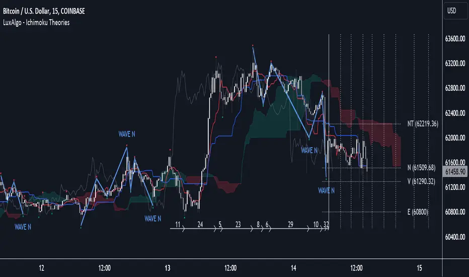
Ichimoku Theories [LuxAlgo]The Ichimoku Theories indicator is the most complete Ichimoku tool you will ever need. Four tools combined into one to harness all the power of Ichimoku Kinkō Hyō.
This tool features the following concepts based on the work of Goichi Hosoda:
Ichimoku Kinkō Hyō: Original Ichimoku indicator with its five main lines and kumo.
Time Theory: automatic time cycle identification and forecasting to understand market timing.
Wave Theory: automatic wave identification to understand market structure.
Price Theory: automatic identification of developing N waves and possible price targets to understand future price behavior.
🔶 ICHIMOKU KINKŌ HYŌ
Ichimoku with lines only, Kumo only and both together
Let us start with the basics: the Ichimoku original indicator is a tool to understand the market, not to predict it, it is a trend-following tool, so it is best used in trending markets.
Ichimoku tells us what is happening in the market and what may happen next, the aim of the tool is to provide market understanding, not trading signals.
The tool is based on calculating the mid-point between the high and low of three pre-defined ranges as the equilibrium price for short (9 periods), medium (26 periods), and long (52 periods) time horizons:
Tenkan sen: middle point of the range of the last 9 candles
Kinjun sen: middle point of the range of the last 26 candles
Senkou span A: middle point between Tankan Sen and Kijun Sen, plotted 26 candles into the future
Senkou span B: midpoint of the range of the last 52 candles, plotted 26 candles into the future
Chikou span: closing price plotted 26 candles into the past
Kumo: area between Senkou pans A and B (kumo means cloud in Japanese)
The most basic use of the tool is to use the Kumo as an area of possible support or resistance.
🔶 TIME THEORY
Current cycles and forecast
Time theory is a critical concept used to identify historical and current market cycles, and use these to forecast the next ones. This concept is based on the Kihon Suchi (translating to "Basic Numbers" in Japanese), these are 9 and 26, and from their combinations we obtain the following sequence:
9, 17, 26, 33, 42, 51, 65, 76, 129, 172, 200, 257
The main idea is that the market moves in cycles with periods set by the Kihon Suchi sequence.
When the cycle has the same exact periods, we obtain the Taito Suchi (translating to "Same Number" in Japanese).
This tool allows traders to identify historical and current market cycles and forecast the next one.
🔹 Time Cycle Identification
Presentation of 4 different modes: SWINGS, HIGHS, KINJUN, and WAVES .
The tool draws a horizontal line at the bottom of the chart showing the cycles detected and their size.
The following settings are used:
Time Cycle Mode: up to 7 different modes
Wave Cycle: Which wave to use when WAVE mode is selected, only active waves in the Wave Theory settings will be used.
Show Time Cycles: keep a cleaner chart by disabling cycles visualisation
Show last X time cycles: how many cycles to display
🔹 Time Cycle Forecast
Showcasing the two forecasting patterns: Kihon Suchi and Taito Suchi
The tool plots horizontal lines, a solid anchor line, and several dotted forecast lines.
The following settings are used:
Show time cycle forecast: to keep things clean
Forecast Pattern: comes in two flavors
Kihon Suchi plots a line from the anchor at each number in the Kihon Suchi sequence.
Taito Suchi plot lines from the anchor with the same size detected in the anchored cycle
Anchor forecast on last X time cycle: traders can place the anchor in any detected cycle
🔶 WAVE THEORY
All waves activated with overlapping
The main idea behind this theory is that markets move like waves in the sea, back and forth (making swing lows and highs). Understanding the current market structure is key to having realistic expectations of what the market may do next. The waves are divided into Simple and Complex.
The following settings are used:
Basic Waves: allows traders to activate waves I, V and N
Complex Waves: allows traders to activate waves P, Y and W
Overlapping waves: to avoid missing out on any of the waves activated
Show last X waves: how many waves will be displayed
🔹 Basic Waves
The three basic waves
The basic waves from which all waves are made are I, V, and N
I wave: one leg moves
V wave: two legs move, one against the other
N wave: Three legs move, push, pull back, and another push
🔹 Complex Waves
Three complex waves
There are other waves like
P wave: contracting market
Y wave: expanding market
W wave: double top or double bottom
🔶 PRICE THEORY
All targets for the current N wave with their calculations
This theory is based on identifying developing N waves and predicting potential price targets based on that developing wave.
The tool displays 4 basic targets (V, E, N, and NT) and 3 extended targets (2E and 3E) according to the calculations shown in the chart above. Traders can enable or disable each target in the settings panel.
🔶 USING EVERYTHING TOGETHER
Please DON'T do this. This is not how you use it
Now the real example:
Daily chart of Nasdaq 100 futures (NQ1!) with our Ichimoku analysis
Time, waves, and price theories go together as one:
First, we identify the current time cycles and wave structure.
Then we forecast the next cycle and possible key price levels.
We identify a Taito Suchi with both legs of exactly 41 candles on each I wave, both together forming a V wave, the last two I waves are part of a developing N wave, and the time cycle of the first one is 191 candles. We forecast this cycle into the future and get 22nd April as a key date, so in 6 trading days (as of this writing) the market would have completed another Taito Suchi pattern if a new wave and time cycle starts. As we have a developing N wave we can see the potential price targets, the price is actually between the NT and V targets. We have a bullish Kumo and the price is touching it, if this Kumo provides enough support for the price to go further, the market could reach N or E targets.
So we have identified the cycle and wave, our expectations are that the current cycle is another Taito Suchi and the current wave is an N wave, the first I wave went for 191 candles, and we expect the second and third I waves together to amount to 191 candles, so in theory the N wave would complete in the next 6 trading days making a swing high. If this is indeed the case, the price could reach the V target (it is almost there) or even the N target if the bulls have the necessary strength.
We do not predict the future, we can only aim to understand the current market conditions and have future expectations of when (time), how (wave), and where (price) the market will make the next turning point where one side of the market overcomes the other (bulls vs bears).
To generate this chart, we change the following settings from the default ones:
Swing length: 64
Show lines: disabled
Forecast pattern: TAITO SUCHI
Anchor forecast: 2
Show last time cycles: 5
I WAVE: enabled
N WAVE: disabled
Show last waves: 5
🔶 SETTINGS
Show Swing Highs & Lows: Enable/Disable points on swing highs and swing lows.
Swing Length: Number of candles to confirm a swing high or swing low. A higher number detects larger swings.
🔹 Ichimoku Kinkō Hyō
Show Lines: Enable/Disable the 5 Ichimoku lines: Kijun sen, Tenkan sen, Senkou span A & B and Chikou Span.
Show Kumo: Enable/Disable the Kumo (cloud). The Kumo is formed by 2 lines: Senkou Span A and Senkou Span B.
Tenkan Sen Length: Number of candles for Tenkan Sen calculation.
Kinjun Sen Length: Number of candles for the Kijun Sen calculation.
Senkou Span B Length: Number of candles for Senkou Span B calculation.
Chikou & Senkou Offset: Number of candles for Chikou and Senkou Span calculation. Chikou Span is plotted in the past, and Senkou Span A & B in the future.
🔹 Time Theory
Show Time Cycle Forecast: Enable/Disable time cycle forecast vertical lines. Disable for better performance.
Forecast Pattern: Choose between two patterns: Kihon Suchi (basic numbers) or Taito Suchi (equal numbers).
Anchor forecast on last X time cycle: Number of time cycles in the past to anchor the time cycle forecast. The larger the number, the deeper in the past the anchor will be.
Time Cycle Mode: Choose from 7 time cycle detection modes: Tenkan Sen cross, Kijun Sen cross, Kumo change between bullish & bearish, swing highs only, swing lows only, both swing highs & lows and wave detection.
Wave Cycle: Choose which type of wave to detect from 6 different wave types when the time cycle mode is set to WAVES.
Show Time Cycles: Enable/Disable time cycle horizontal lines. Disable for better performance.
how last X time cycles: Maximum number of time cycles to display.
🔹 Wave Theory
Basic Waves: Enable/Disable the display of basic waves, all at once or one at a time. Disable for better performance.
Complex Waves: Enable/Disable complex wave display, all at once or one by one. Disable for better performance.
Overlapping Waves: Enable/Disable the display of waves ending on the same swing point.
Show last X waves: 'Maximum number of waves to display.
🔹 Price Theory
Basic Targets: Enable/Disable horizontal price target lines. Disable for better performance.
Extended Targets: Enable/Disable extended price target horizontal lines. Disable for better performance.
Volume Bull/Bear Activity [ZC]Volume Bull/Bear Activity Summary
This indicator generates a summary of bull/bear activity for 20 symbols.
For each symbol, two bars are displayed, colored green and red.
The green bar indicates bull volume, reflecting activity within the last candle of the symbol.
The red bar signifies bear volume within the real-time bar, continuously updated.
You can seamlessly adjust the timeframe for this indicator.
Features :
Bear/Bull Volume bars ( Realtime )
ability to add 20 symbols
price is colored in Green or red to determine if its Green/Red candle .
More into its data

Mxwll Price Action Suite [Mxwll]Introducing the Mxwll Price Action Suite!
The Mxwll Price Action Suite is an all-in-one analysis indicator incorporating elements of SMC and also ideas extending beyond the trading methodology!
Features
Internal structures
External structures
Customizable Sensitivities
BoS/CHoCH
Order Blocks
HH/LH/LL/LH Areas
Rolling TF highs/lows
Rolling Volume Comparisons
Auto Fibs
And more!
The image above shows the indicator's market structure identification capabilities. Internal BoS and CHoCH structures in addition to overarching market structures are available with customizable sensitivities.
The image above shows the indicator identifying order blocks! Additionally, HH/LH/LL/LH areas are also identified.
The image above shows a rolling area of interest. These areas can be compared to supply/demand zones, where traders might consider a bargain long/short/sell area.
The indicator displays a rolling 4hr high/low and 1D high/low, alongside auto fibonacci levels with a customizable sensitivity.
Finally, the Mxwll Price Action Suite shows relevant session information.
Table information
Current Session
Countdown to session close
Next Session
Countdown to next session open
Rolling 4-Hr volume intensity
Rolling 24-Hr volume intensity
Introducing the Mxwll SMC Suite!
The Mxwll SMC Suite is an all-in-one analysis indicator incorporating elements of SMC and also ideas extending beyond the trading methodology!
Features
Internal structures
External structures
Customizable Sensitivities
BoS/CHoCH
Order Blocks
HH/LH/LL/LH Areas
Rolling TF highs/lows
Rolling Volume Comparisons
Auto Fibs
And more!
The image above shows the indicator's market structure identification capabilities. Internal BoS and CHoCH structures in addition to overarching market structures are available with customizable sensitivities.
The image above shows the indicator identifying order blocks! Additionally, HH/LH/LL/LH areas are also identified.
The image above shows a rolling area of interest. These areas can be compared to supply/demand zones, where traders might consider a bargain long/short/sell area.
The indicator displays a rolling 4hr high/low and 1D high/low, alongside auto fibonacci levels with a customizable sensitivity.
Finally, the Mxwll Price Action Suite shows relevant session information.
Table information
Current Session
Countdown to session close
Next Session
Countdown to next session open
Rolling 4-Hr volume intensity
Rolling 24-Hr volume intensity
Expanded Features of Mxwll Price Action Suite
Internal and External Structures
Internal Structures: These elements refer to the price formations and patterns that occur within a smaller scope or a specific trading session. The suite can detect intricate details like minor support/resistance levels or short-term trend reversals.
External Structures: These involve larger, more significant market patterns and trends spanning multiple sessions or time frames. This capability helps traders understand overarching market directions.
Customizable Sensitivities
Adjusting sensitivity settings allows users to tailor the indicator's responsiveness to market changes. Higher sensitivity can catch smaller fluctuations, while lower sensitivity might focus on more significant, reliable market moves.
Break of Structure (BoS) and Change of Character (CHoCH)
BoS: This feature identifies points where the price breaks a significant structure, potentially indicating a new trend or a trend reversal.
CHoCH: Detects subtle shifts in the market's behavior, which could suggest the early stages of a trend change before they become apparent to the broader market.
Order Blocks and Market Phases
Order Blocks: These are essentially price levels or zones where significant trading activities previously occurred, likely pointing to the positions of smart money.
HH/LH/LL/LH Areas: Identifying Higher Highs (HH), Lower Highs (LH), Lower Lows (LL), and Lower Highs (LH) helps in understanding the trend and market structure, aiding in predictive analysis.
Rolling Timeframe Highs/Lows and Volume Comparisons
Tracks highs and lows over specified rolling periods, providing dynamic support and resistance levels.
Compares volume data across different timeframes to assess the strength or weakness of the current price movements.
Auto Fibonacci Levels
Automatically calculates and plots Fibonacci retracement levels, a popular tool among traders to identify potential reversal points based on past movements.
Session Data and Volume Intensity
Session Information: Displays current and upcoming trading sessions along with countdown timers, which is crucial for day traders and those trading on session overlaps.
Volume Intensity: Measures and compares the volume within the last 4 hours and 24 hours to gauge market activity and potential breakout/breakdown movements.
Visualizations and Practical Use
Dynamic Visuals: The suite provides dynamic visual aids, such as real-time updating of high/low markers and Fibonacci levels, which adjust as new data comes in. This feature is critical in fast-paced markets.
Strategic Entry/Exit Points: By identifying order blocks and using Fibonacci levels, traders can pinpoint strategic entry and exit points, maximizing potential returns.
Risk Management: Enhanced features like session countdowns and volume intensity help in better risk management by providing traders with more data on market sentiment and potential volatility.

Percent Rank HistogramThis Pine script indicator is designed to create a visual representation of the percent rank for multiple financial instruments. Here's a breakdown of its key features:
Percent Rank Calculation:
The core functionality of this Pine script indicator revolves around the calculation of the percent rank for each selected financial instrument.
The percent rank is a statistical measure that indicates the percentage of historical data points that are less than or equal to the current value in a given series.
Symbol Selection:
The script allows the user to select up to 10 financial instruments (tickers) for analysis. The default symbols include various cryptocurrencies such as BTCUSD, ETHUSD etc., and TOTAL market cap at ticker 1, to show overal trend of crypto market.
(Top 9 Coins by market cap).
Columns and Colors:
The script visually represents the percent rank using columns based on lines.
The color of each column is determined by a gradient from red to green based on the calculated percent rank, providing a quick visual indication of the instrument's relative performance.
BTC Trending Up while other coins are underperformance:
Labels:
Labels are displayed on the chart, indicating the symbol name and the corresponding percent rank percentage.
The labels include directional arrows (▲ or ▼) to denote whether the percent rank is increasing or decreasing.
Customization:
Users can customize parameters such as the percent rank length and column width to adapt the indicator to their specific preferences, or select needed assets to compare them to each other.
Chart Desk and Scales:
The script includes the visualization of a chart desk with scale lines to provide additional context to the chart. When Percent Rank above middle scale line (50) usually it signaling about asset trending up and below 50 asset trending down.
Mozilla Public License:
The script is subject to the terms of the Mozilla Public License 2.0.
This indicator is useful for traders and analysts interested in visually assessing the percent rank of multiple financial instruments simultaneously, helping them identify potential opportunities or trends in the market.

Heat Map SeasonsHeat Map Seasons indicator
Indicator offers traders a unique perspective on market dynamics by visualizing seasonal trends and deviations from typical price behavior. By blending regression analysis with a color-coded heat map, this indicator highlights periods of heightened volatility and helps identify potential shifts in market sentiment.
Summer:
In the context of the indicator, "summer" represents a period of heightened volatility and upward price momentum in the market. This is analogous to the warmer months of the year when activities are typically more vibrant and energetic. During the "summer" phase indicated by the indicator, traders may observe strong bullish trends, increased trading volumes, and larger price movements. It suggests a favorable environment for bullish strategies, such as trend following or momentum trading. However, traders should exercise caution as heightened volatility can also lead to increased risk and potential drawdowns.
Winter:
Conversely, "winter" signifies a period of decreased volatility and potentially sideways or bearish price action in the market. Similar to the colder months of the year when activities tend to slow down, the "winter" phase in the indicator suggests a quieter market environment with subdued price movements and lower trading volumes. During this phase, traders may encounter choppy price action, consolidation patterns, or even downtrends. It indicates a challenging environment for trend-following strategies and may require a more cautious approach, such as range-bound or mean-reversion trading strategies.
In summary, the "summer" and "winter" phases in the "Heat Map Seasons" indicator provide traders with valuable insights into the prevailing market sentiment and can help inform their trading decisions based on the observed levels of volatility and price momentum.
How to Use:
Watch for price bars that deviate significantly from the regression line , as these may signal potential trading opportunities.
Use the seasonal gauge to gauge the current market sentiment and adjust trading strategies accordingly.
Experiment with different settings for Length and Heat Sensitivity to customize the indicator to your trading style and preferences.
The "Heat Map Seasons" indicator can potentially identify overheated market tops and bottoms on a weekly timeframe by detecting significant deviations from the regression line and observing extreme color gradients in the heat map. Here's how it can be used for this purpose:
Observing Extreme Color Gradients:
When the market is overheated and reaches a potential top, you may observe extremely warm colors (e.g., deep red) in the heat map section of the indicator.
Traders can interpret this as a warning sign of a potential market top, indicating that bullish momentum may be reaching unsustainable levels.
Conversely, when prices deviate too far below the regression line, it may indicate oversold conditions and a potential bottom.
Potential Tops and Bottoms:
User Inputs:
Length: Determines the length of the regression analysis period.
Heat Sensitivity: Controls the sensitivity of the heat map to deviations from the regression line.
Show Regression Line: Option to display or hide the regression line on the chart
Note: This indicator is best used in conjunction with other technical analysis tools and should not be relied upon as the sole basis for trading decisions.

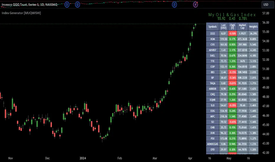
Index Generator [By MUQWISHI]▋ INTRODUCTION :
The “Index Generator” simplifies the process of building a custom market index, allowing investors to enter a list of preferred holdings from global securities. It aims to serve as an approach for tracking performance, conducting research, and analyzing specific aspects of the global market. The output will include an index value, a table of holdings, and chart plotting, providing a deeper understanding of historical movement.
_______________________
▋ OVERVIEW:
The image can be taken as an example of building a custom index. I created this index and named it “My Oil & Gas Index”. The index comprises several global energy companies. Essentially, the indicator weights each company by collecting the number of shares and then computes the market capitalization before sorting them as seen in the table.
_______________________
▋ OUTPUTS:
The output can be divided into 3 sections:
1. Index Title (Name & Value).
2. Index Holdings.
3. Index Chart.
1. Index Title , displays the index name at the top, and at the bottom, it shows the index value, along with the daily change in points and percentage.
2. Index Holdings , displays list the holding securities inside a table that contains the ticker, price, daily change %, market cap, and weight %. Additionally, a tooltip appears when the user passes the cursor over a ticker's cell, showing brief information about the company, such as the company's name, exchange market, country, sector, and industry.
3. Index Chart , display a plot of the historical movement of the index in the form of a bar, candle, or line chart.
_______________________
▋ INDICATOR SETTINGS:
(1) Naming the index.
(2) Entering a currency. To unite all securities in one currency.
(3) Table location on the chart.
(4) Table’s cells size.
(5) Table’s colors.
(6) Sorting table. By securities’ (Market Cap, Change%, Price, or Ticker Alphabetical) order.
(7) Plotting formation (Candle, Bar, or Line)
(8) To show/hide any indicator’s components.
(9) There are 34 fields where user can fill them with symbols.
Please let me know if you have any questions.
Higher-timeframe requests█ OVERVIEW
This publication focuses on enhancing awareness of the best practices for accessing higher-timeframe (HTF) data via the request.security() function. Some "traditional" approaches, such as what we explored in our previous `security()` revisited publication, have shown limitations in their ability to retrieve non-repainting HTF data. The fundamental technique outlined in this script is currently the most effective in preventing repainting when requesting data from a higher timeframe. For detailed information about why it works, see this section in the Pine Script™ User Manual .
█ CONCEPTS
Understanding repainting
Repainting is a behavior that occurs when a script's calculations or outputs behave differently after restarting it. There are several types of repainting behavior, not all of which are inherently useless or misleading. The most prevalent form of repainting occurs when a script's calculations or outputs exhibit different behaviors on historical and realtime bars.
When a script calculates across historical data, it only needs to execute once per bar, as those values are confirmed and not subject to change. After each historical execution, the script commits the states of its calculations for later access.
On a realtime, unconfirmed bar, values are fluid . They are subject to change on each new tick from the data provider until the bar closes. A script's code can execute on each tick in a realtime bar, meaning its calculations and outputs are subject to realtime fluctuations, just like the underlying data it uses. Each time a script executes on an unconfirmed bar, it first reverts applicable values to their last committed states, a process referred to as rollback . It only commits the new values from a realtime bar after the bar closes. See the User Manual's Execution model page to learn more.
In essence, a script can repaint when it calculates on realtime bars due to fluctuations before a bar's confirmation, which it cannot reproduce on historical data. A common strategy to avoid repainting when necessary involves forcing only confirmed values on realtime bars, which remain unchanged until each bar's conclusion.
Repainting in higher-timeframe (HTF) requests
When working with a script that retrieves data from higher timeframes with request.security() , it's crucial to understand the differences in how such requests behave on historical and realtime bars .
The request.security() function executes all code required by its `expression` argument using data from the specified context (symbol, timeframe, or modifiers) rather than on the chart's data. As when executing code in the chart's context, request.security() only returns new historical values when a bar closes in the requested context. However, the values it returns on realtime HTF bars can also update before confirmation, akin to the rollback and recalculation process that scripts perform in the chart's context on the open bar. Similar to how scripts operate in the chart's context, request.security() only confirms new values after a realtime bar closes in its specified context.
Once a script's execution cycle restarts, what were previously realtime bars become historical bars, meaning the request.security() call will only return confirmed values from the HTF on those bars. Therefore, if the requested data fluctuates across an open HTF bar, the script will repaint those values after it restarts.
This behavior is not a bug; it's simply the default behavior of request.security() . In some cases, having the latest information from an unconfirmed HTF bar is precisely what a script needs. However, in many other cases, traders will require confirmed, stable values that do not fluctuate across an open HTF bar. Below, we explain the most reliable approach to achieve such a result.
Achieving consistent timing on all bars
One can retrieve non-fluctuating values with consistent timing across historical and realtime feeds by exclusively using request.security() to fetch the data from confirmed HTF bars. The best way to achieve this result is offsetting the `expression` argument by at least one bar (e.g., `close [1 ]`) and using barmerge.lookahead_on as the `lookahead` argument.
We discourage the use of barmerge.lookahead_on alone since it prompts the function to look toward future values of HTF bars across historical data, which is heavily misleading. However, when paired with a requested `expression` that includes a one-bar historical offset, the "future" data the function retrieves is not from the future. Instead, it represents the last confirmed bar's values at the start of each HTF bar, thus preventing the results on realtime bars from fluctuating before confirmation from the timeframe.
For example, this line of code uses a request.security() call with barmerge.lookahead_on to request the close price from the "1D" timeframe, offset by one bar with the history-referencing operator [ ] . This line will return the daily price with consistent timing across all bars:
float htfClose = request.security(syminfo.tickerid, "1D", close , lookahead = barmerge.lookahead_on)
Note that:
• This technique only works as intended for higher-timeframe requests .
• When designing a script to work specifically with HTFs, we recommend including conditions to prevent request.security() from accessing timeframes equal to or lower than the chart's timeframe, especially if you intend to publish it. In this script, we included an if structure that raises a runtime error when the requested timeframe is too small.
• A necessary trade-off with this approach is that the script must wait for an HTF bar's confirmation to retrieve new data on realtime bars, thus delaying its availability until the open of the subsequent HTF bar. The time elapsed during such a delay varies with each market, but it's typically relatively small.
👉 Failing to offset the function's `expression` argument while using barmerge.lookahead_on will produce historical results with lookahead bias , as it will look to the future states of historical HTF bars, retrieving values before the times at which they're available in the feed. See the `lookahead` and Future leak with `request.security()` sections in the Pine Script™ User Manual for more information.
Evolving practices
The fundamental technique outlined in this publication is currently the only reliable approach to requesting non-repainting HTF data with request.security() . It is the superior approach because it avoids the pitfalls of other methods, such as the one introduced in the `security()` revisited publication. That publication proposed using a custom `f_security()` function, which applied offsets to the `expression` and the requested result based on historical and realtime bar states. At that time, we explored techniques that didn't carry the risk of lookahead bias if misused (i.e., removing the historical offset on the `expression` while using lookahead), as requests that look ahead to the future on historical bars exhibit dangerously misleading behavior.
Despite these efforts, we've unfortunately found that the bar state method employed by `f_security()` can produce inaccurate results with inconsistent timing in some scenarios, undermining its credibility as a universal non-repainting technique. As such, we've deprecated that approach, and the Pine Script™ User Manual no longer recommends it.
█ METHOD VARIANTS
In this script, all non-repainting requests employ the same underlying technique to avoid repainting. However, we've applied variants to cater to specific use cases, as outlined below:
Variant 1
Variant 1, which the script displays using a lime plot, demonstrates a non-repainting HTF request in its simplest form, aligning with the concept explained in the "Achieving consistent timing" section above. It uses barmerge.lookahead_on and offsets the `expression` argument in request.security() by one bar to retrieve the value from the last confirmed HTF bar. For detailed information about why this works, see the Avoiding Repainting section of the User Manual's Other timeframes and data page.
Variant 2
Variant 2 ( fuchsia ) introduces a custom function, `htfSecurity()`, which wraps the request.security() function to facilitate convenient repainting control. By specifying a value for its `repaint` parameter, users can determine whether to allow repainting HTF data. When the `repaint` value is `false`, the function applies lookahead and a one-bar offset to request the last confirmed value from the specified `timeframe`. When the value is `true`, the function requests the `expression` using the default behavior of request.security() , meaning the results can fluctuate across chart bars within realtime HTF bars and repaint when the script restarts.
Note that:
• This function exclusively handles HTF requests. If the requested timeframe is not higher than the chart's, it will raise a runtime error .
• We prefer this approach since it provides optional repainting control. Sometimes, a script's calculations need to respond immediately to realtime HTF changes, which `repaint = true` allows. In other cases, such as when issuing alerts, triggering strategy commands, and more, one will typically need stable values that do not repaint, in which case `repaint = false` will produce the desired behavior.
Variant 3
Variant 3 ( white ) builds upon the same fundamental non-repainting approach used by the first two. The difference in this variant is that it applies repainting control to tuples , which one cannot pass as the `expression` argument in our `htfSecurity()` function. Tuples are handy for consolidating `request.*()` calls when a script requires several values from the same context, as one can request a single tuple from the context rather than executing multiple separate request.security() calls.
This variant applies the internal logic of our `htfSecurity()` function in the script's global scope to request a tuple containing open and `srcInput` values from a higher timeframe with repainting control. Historically, Pine Script™ did not allow the history-referencing operator [ ] when requesting tuples unless the tuple came from a function call, which limited this technique. However, updates to Pine over time have lifted this restriction, allowing us to pass tuples with historical offsets directly as the `expression` in request.security() . By offsetting all items in a tuple `expression` by one bar and using barmerge.lookahead_on , we effectively retrieve a tuple of stable, non-repainting HTF values.
Since we cannot encapsulate this method within the `htfSecurity()` function and must execute the calculations in the global scope, the script's "Repainting" input directly controls the global `offset` and `lookahead` values to ensure it behaves as intended.
Variant 4 (Control)
Variant 4, which the script displays as a translucent orange plot, uses a default request.security() call, providing a reference point to compare the difference between a repainting request and the non-repainting variants outlined above. Whenever the script restarts its execution cycle, realtime bars become historical bars, and the request.security() call here will repaint the results on those bars.
█ Inputs
Repainting
The "Repainting" input (`repaintInput` variable) controls whether Variant 2 and Variant 3 are allowed to use fluctuating values from an unconfirmed HTF bar. If its value is `false` (default), these requests will only retrieve stable values from the last confirmed HTF bar.
Source
The "Source" input (`srcInput` variable) determines the series the script will use in the `expression` for all HTF data requests. Its default value is close .
HTF Selection
This script features two ways to specify the higher timeframe for all its data requests, which users can control with the "HTF Selection" input (`tfTypeInput` variable):
1) If its value is "Fixed TF", the script uses the timeframe value specified by the "Fixed Higher Timeframe" input (`fixedTfInput` variable). The script will raise a runtime error if the selected timeframe is not larger than the chart's.
2) If the input's value is "Multiple of chart TF", the script multiplies the value of the "Timeframe Multiple" input (`tfMultInput` variable) by the chart's timeframe.in_seconds() value, then converts the result to a valid timeframe string via timeframe.from_seconds() .
Timeframe Display
This script features the option to display an "information box", i.e., a single-cell table that shows the higher timeframe the script is currently using. Users can toggle the display and determine the table's size, location, and color scheme via the inputs in the "Timeframe Display" group.
█ Outputs
This script produces the following outputs:
• It plots the results from all four of the above variants for visual comparison.
• It highlights the chart's background gray whenever a new bar starts on the higher timeframe, signifying when confirmations occur in the requested context.
• To demarcate which bars the script considers historical or realtime bars, it plots squares with contrasting colors corresponding to bar states at the bottom of the chart pane.
• It displays the higher timeframe string in a single-cell table with a user-specified size, location, and color scheme.
Look first. Then leap.

Trailing Management (Zeiierman)█ Overview
The Trailing Management (Zeiierman) indicator is designed for traders who seek an automated and dynamic approach to managing trailing stops. It helps traders make systematic decisions regarding when to enter and exit trades based on the calculated risk-reward ratio. By providing a clear visual representation of trailing stop levels and risk-reward metrics, the indicator is an essential tool for both novice and experienced traders aiming to enhance their trading discipline.
The Trailing Management (Zeiierman) indicator integrates a Break-Even Curve feature to enhance its utility in trailing stop management and risk-reward optimization. The Break-Even Curve illuminates the precise point at which a trade neither gains nor loses value, offering clarity on the risk-reward landscape. Furthermore, this precise point is calculated based on the required win rate and the risk/reward ratio. This calculation aids traders in understanding the type of strategy they need to employ at any given time to be profitable. In other words, traders can, at any given point, assess the kind of strategy they need to utilize to make money, depending on the price's position within the risk/reward box.
█ How It Works
The indicator operates by computing the highest high and the lowest low over a user-defined period and then applying this information to determine optimal trailing stop levels for both long and short positions.
Directional Bias:
It establishes the direction of the market trend by comparing the index of the highest high and the lowest low within the lookback period.
Bullish
Bearish
Trailing Stop Adjustment:
The trailing stops are adjusted using one of three methods: an automatic calculation based on the median of recent peak differences, pivot points, or a fixed percentage defined by the user.
The Break-Even Curve:
The Break-Even Curve, along with the risk/reward ratio, is determined through the trailing method. This approach utilizes the current closing price as a hypothetical entry point for trades. All calculations, including those for the curve, are based on this current closing price, ensuring real-time accuracy and relevance. As market conditions fluctuate, the curve dynamically adjusts, offering traders a visual benchmark that signifies the break-even point. This real-time adjustment provides traders with an invaluable tool, allowing them to visually track how shifts in the market could impact the point at which their trades neither gain nor lose value.
Example:
Let's say the price is at the midpoint of the risk/reward box; this means that the risk/reward ratio should be 1:1, and the minimum win rate is 50% to break even.
In this example, we can see that the price is near the stop-loss level. If you are about to take a trade in this area and would respect your stop, you only need to have a minimum win rate of 11% to earn money, given the risk/reward ratio, assuming that you hold the trade to the target.
In other words, traders can, at any given point, assess the kind of strategy they need to employ to make money based on the price's position within the risk/reward box.
█ How to Use
Market Bias:
When using the Auto Bias feature, the indicator calculates the underlying market bias and displays it as either bullish or bearish. This helps traders align their trades with the underlying market trend.
Risk Management:
By observing the plotted trailing stops and the risk-reward ratios, traders can make strategic decisions to enter or exit positions, effectively managing the risk.
Strategy selection:
The Break-Even Curve is a powerful tool for managing risk, allowing traders to visualize the relationship between their trailing stops and the market's price movements. By understanding where the break-even point lies, traders can adjust their strategies to either lock in profits or cut losses.
Based on the plotted risk/reward box and the location of the price within this box, traders can easily see the win rate required by their strategy to make money in the long run, given the risk/reward ratio.
Consider this example: The market is bullish, as indicated by the bias, and the indicator suggests looking into long trades. The price is near the top of the risk/reward box, which means entering the market right now carries a huge risk, and the potential reward is very low. To take this trade, traders must have a strategy with a win rate of at least 90%.
█ Settings
Trailing Method:
Auto: The indicator calculates the trailing stop dynamically based on market conditions.
Pivot: The trailing stop is adjusted to the highest high (long positions) or lowest low (short positions) identified within a specified lookback period. This method uses the pivotal points of the market to set the trailing stop.
Percentage: The trailing stop is set at a fixed percentage away from the peak high or low.
Trailing Size (prd):
This setting defines the lookback period for the highest high and lowest low, which affects the sensitivity of the trailing stop to price movements.
Percentage Step (perc):
If the 'Percentage' method is selected, this setting determines the fixed percentage for the trailing stop distance.
Set Bias (bias):
Allows users to set a market bias which can be Bullish, Bearish, or Auto, affecting how the trailing stop is adjusted in relation to the market trend.
-----------------
Disclaimer
The information contained in my Scripts/Indicators/Ideas/Algos/Systems does not constitute financial advice or a solicitation to buy or sell any securities of any type. I will not accept liability for any loss or damage, including without limitation any loss of profit, which may arise directly or indirectly from the use of or reliance on such information.
All investments involve risk, and the past performance of a security, industry, sector, market, financial product, trading strategy, backtest, or individual's trading does not guarantee future results or returns. Investors are fully responsible for any investment decisions they make. Such decisions should be based solely on an evaluation of their financial circumstances, investment objectives, risk tolerance, and liquidity needs.
My Scripts/Indicators/Ideas/Algos/Systems are only for educational purposes!
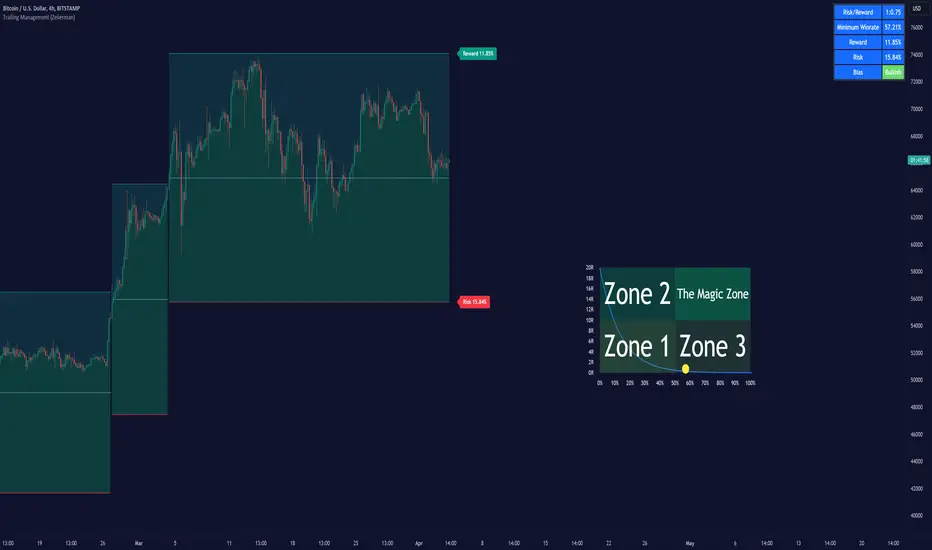
Periodic Activity Tracker [LuxAlgo]The Periodic Activity Tracker tool periodically tracks the cumulative buy and sell volume in a user-defined period and draws the corresponding matching bars and volume delta for each period.
Users can select a predefined aggregation period from the following options: Hourly, Daily, Weekly, and Monthly.
🔶 USAGE
This tool provides a simple and clear way of analyzing volumes for each aggregated period and is made up of the following elements:
Buy and sell volumes by period as red and green lines with color gradient area
Delta (difference) between buy & sell volume for each period
Buy & sell volume bars for each period
Separator between lines and bars, and period tags below each pair of bars for ease of reading
On the chart above we can see all the elements displayed, the volume level on the lines perfectly matches the volume level on the bars for each period.
In this case, the tool has the default settings so the anchor period is set to Daily and we can see how the period tag (each day of the week) is displayed below each pair of bars.
Users can disable the delta display and adjust the bar size.
🔹 Reading The Tool
In trading, assessing the strength of the bulls (buyers) and bears (sellers) is key to understanding the current trading environment. Which side, if any, has the upper hand? To answer this question, some traders look at volume in relation to price.
This tool provides you with a view of buy volume versus sell volume, allowing you to compare both sides of the market.
As with any volume tool, the key is to understand when the forces of the two groups are balanced or unbalanced.
As we can observe on the chart:
NOV '23: Buy volume greater than sell volume, both moving up close together, flat delta. We can see that the price is in range.
DEC '23: Buy volume bigger than Sell volume, both moving up but with a bigger difference, bigger delta than last month but still flat. We can see the price in the range above last month's range.
JAN '24: Buy and sell volume tied together, no delta whatsoever. We can see the price in range but testing above and below last month's range.
FEB '24: Buy volume explodes higher and sell volume cannot keep up, big growing delta. Price explodes higher above last month's range.
Traders need to understand that there is always an equal number of buyers and sellers in a liquid market, the quality here is how aggressive or passive they are. Who is 'attacking' and who is 'defending', who is using market orders to move prices, and who is using limit orders waiting to be filled?
This tool gives you the following information:
Lines: if the top line is green, the buyers are attacking, if it is red, the sellers are attacking.
Delta: represents the difference in their strength, if it is above 0 the buyers are stronger, if it is below 0 the sellers are stronger.
Bars: help you to see the difference in strength between buyers and sellers for each period at a glance.
🔹 Anchor Period
By default, the tool is set to Hourly. However, users can select from a number of predefined time periods.
Depending on the user's selection, the bars are displayed as follows:
Hourly : hours of the current day
Daily : days of the current week
Weekly : weeks of the current month
Monthly : months of the current year
On the chart above we can see the four periods displayed, starting at the top left and moving clockwise we have hourly, daily, weekly, and monthly.
🔶 DETAILS
🔹 Chart TimeFrame
The chart timeframe has a direct impact on the visualization of the tool, and the user should select a chart timeframe that is compatible with the Anchor period in the tool's settings panel.
For the chart timeframe to be compatible it must be less than the Anchor period parameter. If the user selects an incompatible chart timeframe, a warning message will be displayed.
As a rule of thumb, the smaller the chart timeframe, the more data the tool will collect, returning indications for longer-term price variations.
These are the recommended chart timeframes for each period:
Hourly : 5m charts or lower
Daily : 1H charts or lower
Weekly : 4H charts or lower
Monthly : 1D charts or lower
🔹 Warnings
This chart shows both types of warnings the user may receive
At the top, we can see the warning that is given when the 'Bar Width' parameter exceeds the allowed value.
At the bottom is the incompatible chart timeframe warning, which prompts the user to select a smaller chart timeframe or a larger "Anchor Period" parameter.
🔶 SETTINGS
🔹 Data Gathering
Anchor period: Time period representing each bar: hours of the day, days of the week, weeks of the month, and months of the year. The timeframe of the chart must be less than this parameter, otherwise a warning will be displayed.
🔹 Style
Bars width: Size of each bar, there is a maximum limit so a warning will be displayed if it is reached.
Volume color
Delta: Enable/Disable Delta Area Display
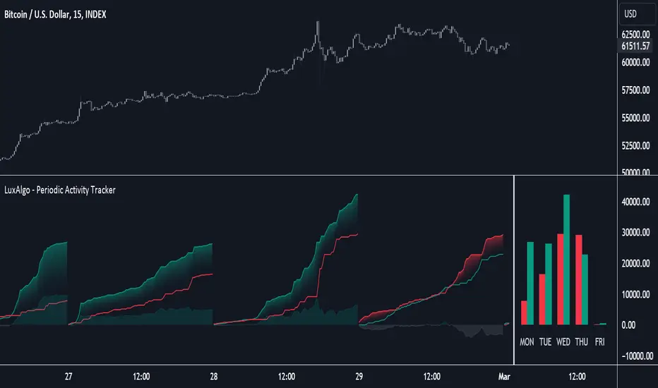
Gaps Profile [vnhilton]Note: If you get an error preventing indicator from executing due to a loop running longer than >500ms, please lower the amount of boxes shown and/or increase the minimum gap % threshold.
OVERVIEW
The Gaps Profile (GP) simply shows the remaining gaps on the chart that have yet to be closed. Gaps are created where there's a distance between the current open and the previous close. Big gaps suggest change in sentiment and volatility causing prices to pull away thereby creating gaps. Gaps can be used as pivot areas where price may attempt to close the inefficiency entirely and/or serve as supply/demand zones.
(FEATURES)
- 3 to 499 remaining up/down gaps can be displayed on the chart (furthest gaps away from price are removed to make way for new gaps)
- Minimum gap % threshold
- Ability to highlight largest or newest up/down gap
- 4 GP color themes: Mono, Up/Down, Up/Down Largest Gradients, Up/Down Newest Gradients
- GP Type: Left, Right (how it is built - overlapping gaps plotted from left/right to right/left)
- GP offset from current bar
- Box border width
- Box border style for up/down: Dashed, Dotted, Solid
- Toggles to hide border/box with ease

TTrades Daily Bias [TFO]Inspired by @TTrades_edu video on daily bias, this indicator aims to develop a higher timeframe bias and collect data on its success rate. While a handful of concepts were introduced in said video, this indicator focuses on one specific method that utilizes previous highs and lows. The following description will outline how the indicator works using the daily timeframe as an example, but the weekly timeframe is also an included option that functions in the exact same manner.
On the daily timeframe, there are a handful of possible scenarios that we consider: if price closes above its previous day high (PDH), the following day's bias will target PDH; if price trades above its PDH but closes back below it, the following day's bias will target its previous day low (PDL).
Similarly, if price closes below its PDL, the following day's bias will target PDL. If price trades below its PDL but closes back above it, the following day's bias will target PDH.
If price trades as an inside bar that doesn't take either PDH or PDL, it will refer to the previous candle for bias. If the previous day closed above its open, it will target PDH and vice versa. If price trades as an outside bar that takes both PDH and PDL, but closes inside that range, no bias is assigned.
With a rigid framework in place, we can apply it to the charts and observe the results.
As shown above, each new day starts by drawing out the PDH and PDL levels. They start out as blue and turn red once traded through (these are the default colors which can be changed in the indicator's settings). The triangles you see are plotted to indicate the time at which PDH or PDL was traded through. This color scheme is also applied to the table in the top right; once a bias is determined, that cell's color starts out as blue and turns red once the level is traded through.
The table indicates the success rate of price hitting the levels provided by each period's bias, followed by the success rate of price closing through said levels after reaching them, as well as the sample size of data collected for each scenario.
In the above crude oil futures (CL1!) 30m chart, we can glean a lot of information from the table in the top right. First we may note that the "PDH" cell is red, which indicates that the current day's bias was targeting PDH and it has already traded through that level. We might also note that the "PWH" cell is blue, which indicates that the weekly bias is targeting the previous week high (PWH) but price has yet to reach that level.
As an example of how to read the table's data, we can look at the "PDH" row of the crude oil chart above. The sample size here indicates that there were 279 instances where the daily bias was assigned as PDH. From this sample size, 76.7% of instances did go on to trade through PDH, and only 53.7% of those instances actually went on to close through PDH after hitting that level.
Of course, greater sample sizes and therefore greater statistical significance may be derived from higher timeframe charts that may go further back in time. The amount of data you can observe may also depend on your TradingView plan.
If we don't want to see the labels describing why bias is assigned a certain way, we can simply turn off the "Show Bias Reasoning" option. Additionally, if we want to see a visual of what the daily and weekly bias currently is, we can plot that along the top and bottom of the chart, as shown above. Here I have daily bias plotted at the top and weekly bias at the bottom, where the default colors of green and red indicate that the bias logic is expecting price to draw towards the given timeframe's previous high or low, respectively.
For a compact table view that doesn't take up much chart space, simply deselect the "Show Statistics" option. This will only show the color-coded bias column for a quick view of what levels are being anticipated (more user-friendly for mobile and other smaller screens).
Alerts can be configured to indicate the bias for a new period, and/or when price hits its previous highs and lows. Simply enable the alerts you want from the indicator's settings and create a new alert with this indicator as the condition. There will be options to use "Any alert() function call" which will alert whatever is selected from the settings, or you can use more specific alerts for bullish/bearish bias, whether price hit PDH/PDL, etc.
Lastly, while the goal of this indicator was to evaluate the effectiveness of a very specific bias strategy, please understand that past performance does not guarantee future results.
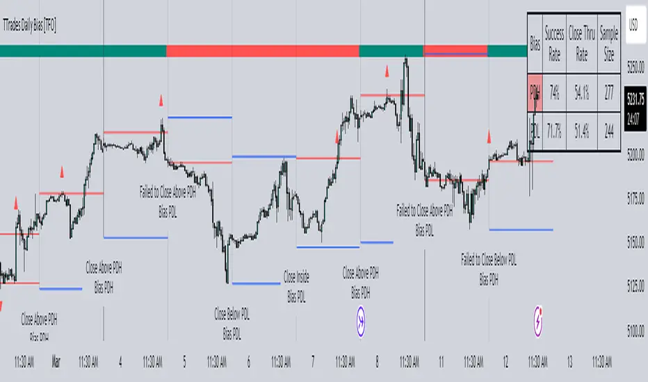
Risk Management Chart█ OVERVIEW
Risk Management Chart allows you to calculate and visualize equity and risk depend on your risk-reward statistics which you can set at the settings.
This script generates random trades and variants of each trade based on your settings of win/loss percent and shows it on the chart as different polyline and also shows thick line which is average of all trades.
It allows you to visualize and possible to analyze probability of your risk management. Be using different settings you can adjust and change your risk management for better profit in future.
It uses compound interest for each trade.
Each variant of trade is shown as a polyline with color from gradient depended on it last profit.
Also I made blurred lines for better visualization with function :
poly(_arr, _col, _t, _tr) =>
for t = 1 to _t
polyline.new(_arr, false, false, xloc.bar_index, color.new(_col, 0 + t * _tr), line_width = t)
█ HOW TO USE
Just add it to the cart and expand the window.
█ SETTINGS
Start Equity $ - Amount of money to start with (your equity for trades)
Win Probability % - Percent of your win / loss trades
Risk/Reward Ratio - How many profit you will get for each risk(depends on risk per trade %)
Number of Trades - How many trades will be generated for each variant of random trading
Number of variants(lines) - How many variants will be generated for each trade
Risk per Trade % -risk % of current equity for each trade
If you have any ask it at comments.
Hope it will be useful.