Educational

EPS and Sales Magic Indicator V2EPS and Sales Magic Indicator V2
EPS and Sales Magic Indicator V2
Short Title: EPS V2
Author: Trading_Tomm
Platform: TradingView (Pine Script v6)
License: Free for public use under fair usage guidelines
Overview
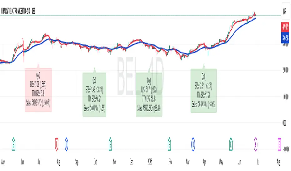
The EPS and Sales Magic Indicator V2 is a powerful stock fundamental visualization tool built specifically for TradingView users who wish to incorporate earnings intelligence directly onto their price chart. Designed and developed by Trading_Tomm, this upgraded version of the original 'EPS and Sales Magic Indicator' includes an enriched and more insightful presentation of company performance metrics — now with TTM EPS support, advanced color-coding, label sizing, and refined control options.
This indicator is tailored for retail traders, swing investors, and long-term fundamental analysts who need to view Quarter-over-Quarter (QoQ) earnings and revenue changes directly on the price chart without switching tabs or breaking focus.
What Does It Display?
The EPS and Sales Magic Indicator V2 intelligently detects quarterly financial updates and displays the following data points via labels:
1. EPS (Earnings Per Share) – Current Quarterly Value
This is the most recent Diluted EPS published by the company, fetched using TradingView’s request.financial() function.
Displayed in the format: EPS: ₹20.45
2. EPS QoQ Percentage Change
Shows the percentage change in EPS compared to the previous quarter.
Highlights improvement or decline using arrows (up for improvement, down for decline).
Displayed in the format: EPS: ₹20.45 (up 15.3 percent)
3. Sales (Revenue) – Current Quarterly Value
Fetches and displays Total Revenue of the company in ₹Crores for easier Indian-market readability.
Displayed in the format: Sales: ₹460Cr
4. Sales QoQ Percentage Change
Measures and presents the quarter-over-quarter percentage change in total revenue.
Uses arrows to indicate growth or contraction.
Displayed in the format: Sales: ₹460Cr (down 3.8 percent)
5. EPS TTM (Trailing Twelve Months)
You now get the TTM EPS — the sum of the last four quarterly EPS values.
This value provides a better long-term earnings snapshot compared to a single quarter.
Displayed in the format: TTM EPS: ₹78.12
All of these values are automatically calculated and displayed only on the bars where a new financial report is detected, keeping your chart clean and insightful.
Customization Features
This indicator is built with user control in mind, allowing you to personalize how and what you want to see:
Show EPS in Label: Enable or disable the display of EPS and EPS QoQ values.
Show Sales in Label: Toggle the visibility of revenue and sales change percentage.
Color Options for Label Themes: The label background color is automatically determined based on performance.
Green: Both EPS and Sales increased QoQ.
Red: Both decreased.
Orange: One increased and the other decreased.
Gray: Default color (if values are unavailable or mixed).
Label Text Size: Choose from Tiny, Small (default), or Normal.
Visual Design
Placement: The labels are positioned just below the candlesticks using yloc.belowbar, so they do not obstruct price action or interfere with technical indicators.
Anchor: Aligned precisely with the financial reporting bars to maintain clarity in historical comparisons.
Background Style: Clean, semi-transparent styling with soft text colors for comfortable viewing.
How It Works
The indicator relies on TradingView’s powerful request.financial() function to extract fiscal quarterly financials (FQ). Internally, it uses detection logic to identify fresh data updates by comparing current vs. previous values, arithmetic to compute QoQ percentage changes in EPS and Sales, logic to build formatted labels dynamically based on user selections, and conditional color and sizing logic to enhance interpretability.
Use Cases
For Long-Term Investors: Quickly identify if a company’s profitability and revenue are improving over time.
For Swing Traders: Combine recent earnings trends with price action to evaluate if post-result momentum has real backing.
For Technical and Fundamental Traders: Layer it with moving averages, RSI, or volume to create a hybrid analysis environment.
Limitations and Notes
Financial data is provided by TradingView’s financial API, and occasional missing values may occur for less-covered stocks.
This tool does not repaint but depends on the timing of the official financial updates.
All values are rounded and formatted to prioritize readability.
Works best on Daily or higher timeframes (weekly or monthly also supported).
License and Fair Use
This script is free to use and share under TradingView’s open-use guidelines. You may copy, fork, and build upon this indicator for personal or educational purposes, but commercial usage requires attribution to the author: Trading_Tomm.
Future Enhancements (Planned)
Addition of Net Profit (QoQ and TTM)
Inclusion of Operating Margin, Profit Margin, and Book Value
Option to switch between numeric and graphical display (table mode)
Alerts on extreme earnings deviation or sales slumps
Final Thoughts
The EPS and Sales Magic Indicator V2 represents a clean, visual, and smart way to monitor a company’s core performance from your chart screen. It helps you align fundamental strength with technical strategies and provides instant financial clarity, which is especially vital in today’s fast-moving markets.
Whether you’re preparing for an earnings season or scanning past performance to pick your next investment, this indicator saves time, enhances insights, and sharpens decisions.
Breakfast RangesJust a range background for Asian, London and New York sessions. I use it to marke the timezone for when i would analyse charts (asian), and when the London and New York sessions start, to see the higher volume and price action come in.


8 EMA vs 21 EMA Crossover AlertsThis indicator creates a Buy signal when 8 EMA crosses above 21 EMA and vice versa on any time frame selected on the chart

Price-EMA Z-Score Backgroundhe “Price‑to‑EMA Z‑Score Background” indicator is designed to give you a clear, visual sense of when price has moved unusually far away from its smoothed trend, and to highlight those moments as potential overextension or mean‑reversion opportunities. Under the hood, it first computes a standard exponential moving average (EMA) of your chosen lookback length, then measures the raw difference between the current close and that EMA on every bar. To make that raw deviation comparable across different markets and timeframes, it converts the series of differences into a z‑score—subtracting the rolling mean of the deviations and dividing by their rolling standard deviation over a second lookback window.
Once you’ve normalized price‑to‑EMA distance into z‑score units, you can set two simple trigger levels: one upper threshold and one lower threshold. Whenever the z‑score climbs above the upper threshold, the chart background glows green, signaling that price is extended far above its EMA (and might be ripe for a pullback). Whenever the z‑score falls below the lower threshold, the background turns red, calling out an equally extreme move below the EMA (and a possible oversold bounce). Between those bands, no shading appears, letting you know price is trading within its “normal” range around the trend.
By adjusting the EMA period, the z‑score lookback, and the two trigger levels, you can dial in early warning signals (e.g. ±1 σ) or wait for very stretched moves (±2 σ or more). Used in concert with your favorite momentum or pattern tools—or even as a standalone visual cue—this simple background‑shading approach makes it easy to spot when a market is running too hot or too cold relative to its own recent average.
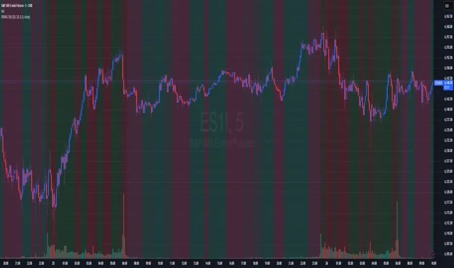
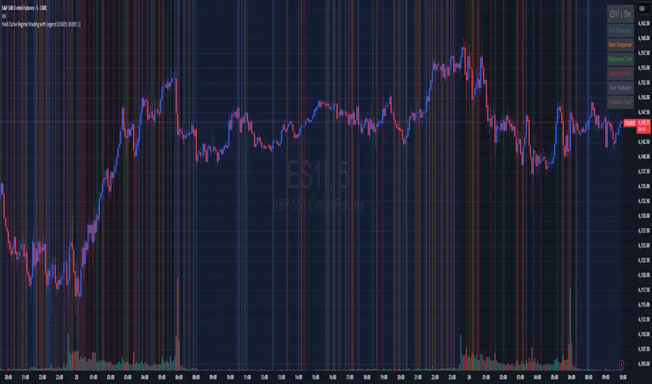
Yield Curve Regime Shading with LegendTakes two symbols (e.g. two futures contracts, two FX pairs, etc.) as inputs.
Calculates the “regime” as the sign of the change in their difference over an n‑period lookback.
Lets you choose whether you want to color the bars themselves or shade the background.
How it works
Inputs
symbolA, symbolB: the two tickers you’re comparing.
n: lookback in bars to measure the change in the spread.
mode: pick between “Shading” or “Candle Color”.
Data fetching
We use request.security() to pull each series at the chart’s timeframe.
Regime calculation
spread = priceA – priceB
spreadPrev = ta.valuewhen(not na(spread), spread , 0) (i.e. the spread n bars ago)
If spread > spreadPrev → bullish regime
If spread < spreadPrev → bearish regime
Plotting
Shading: apply bgcolor() in green/red.
Candle Color: use barcolor() to override the bar color.
Rolling Correlation (Forex)//@version=5
indicator("Rolling Correlation (Forex)", shorttitle="ρ-Corr", overlay = false)
// ── User inputs ────────────────────────────────────────────────────────────────
sym1 = input.symbol("FX_IDC:EURUSD", "First symbol") // Change if your broker uses another prefix
sym2 = input.symbol("FX_IDC:GBPUSD", "Second symbol")
len = input.int(20, "Look-back length", minval = 2)
// ── Pull closing prices from both symbols on the chart’s timeframe ────────────
p1 = request.security(sym1, timeframe.period, close,
barmerge.gaps_off, barmerge.lookahead_on)
p2 = request.security(sym2, timeframe.period, close,
barmerge.gaps_off, barmerge.lookahead_on)
// ── Convert to log-returns (removes price-level bias) ─────────────────────────
r1 = math.log(p1 / p1 )
r2 = math.log(p2 / p2 )
// ── Rolling Pearson correlation ───────────────────────────────────────────────
corr = ta.correlation(r1, r2, len)
// ── Plot ──────────────────────────────────────────────────────────────────────
plot(corr, title = "ρ", linewidth = 2)
hline( 1, "+1 (perfect)", color = color.green)
hline( 0, "0", color = color.gray)
hline(-1, "-1 (inverse)", color = color.red)

VWAP + EMA StrategyUses Vwap and Ema for buy and sell signal. Just looking through and exploring what code can do. Not a financial advice

London & NY Sessions - Full ViewThis Pine Script highlights the London and New York trading sessions on a 5-minute chart using the London time zone. It includes:
✅ A green vertical line and label at London Open (08:00)
✅ A red vertical line and label at New York Open (13:30)
✅ Light green background during the London session (08:00–17:00)
✅ Light red background during the New York session (13:30–21:00)
Use it to visually track key market openings and identify high-volume trading periods.

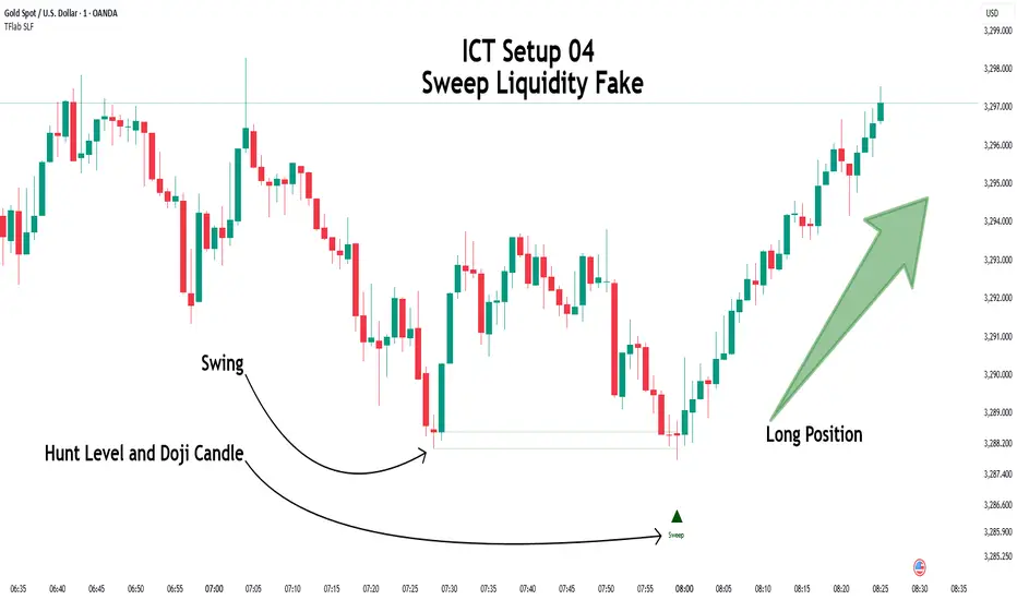
ICT Setup 04 [TradingFinder] SFP Sweep Liquidity Fake CHoCH/BOS🔵 Introduction
In smart money and ICT based trading, liquidity is never random. Some of the most meaningful market moves begin with a liquidity sweep where price intentionally hunts a previous swing high or swing low to trigger stop loss orders and absorb volume.
This manipulation is often followed by a sharp reversal from a reaction zone, creating ideal conditions for a high probability entry. This indicator is built to detect exactly that. It identifies a valid swing point and defines a reaction zone where price is likely to react.
For short setups, the zone lies between the swing high and the maximum of the candle’s open or close. For long setups, it’s drawn from the swing low to the minimum of the open or close.
When price returns to this zone and forms a qualified confirmation candle typically a doji or a small bodied candle that closes inside the zone while sweeping the liquidity this is a potential sign of reversal.
The candle must show both the sweep and the inability to hold above or below the key level, signaling a fake breakout or failed move. By combining elements of liquidity hunt, reaction zone rejection, and candle based entry confirmation, this tool highlights sniper entry points used by smart money to trap retail traders and reverse the trend. It helps filter out noise and enhances timing, making it ideal for trading in alignment with institutional order flow.
Long Position :
Short Position :
🔵 How to Use
This indicator is designed to highlight precise moments where price sweeps liquidity and reacts within a high probability reversal zone. By identifying clean swing highs and lows and defining a smart reaction zone around them, it filters out weak fakeouts and focuses only on setups with strong institutional footprints.
The tool works best when combined with market structure analysis and is suitable for both scalping and intraday trading. Below is a breakdown of how to interpret the signals for long and short positions based on the visual setups provided.
🟣 Long Setup
In a long setup, the indicator first detects a valid swing low where liquidity has likely accumulated below. A reaction zone is then drawn between the swing low and the minimum of the open or close of the swing candle.
When price returns to this zone, it must sweep the previous low and form a precise confirmation candle, such as a doji or a small bodied candle, that closes inside the zone. This candle must also reject the lower level, showing failure to continue downward.
As shown in the chart, once the liquidity grab is complete and the confirmation candle forms, a clean long signal is issued, indicating a potential bullish reversal backed by smart money behavior.
🟣 Short Setup
In a short setup, the indicator identifies a swing high where buy-side liquidity is resting. It then constructs a reaction zone between the high and the maximum of the open or close of the swing candle. Price must return to this zone, sweep the swing high, and form a bearish confirmation candle inside the zone.
A classic example is a doji or rejection candle that traps breakout buyers and fails to hold above the previous high. In the provided chart, the price aggressively hunts the liquidity above the swing high, but the close within the reaction zone signals exhaustion, prompting a short signal with high reversal probability.
These setups represent moments where price action, liquidity behavior, and candle structure align to offer strong entries. By focusing on clean sweeps and reactive confirmations, the indicator helps traders stay on the side of smart money and avoid common breakout traps.
🔵 Settings
🟣 Logical settings
Swing period : You can set the swing detection period.
Max Swing Back Method : It is in two modes "All" and "Custom". If it is in "All" mode, it will check all swings, and if it is in "Custom" mode, it will check the swings to the extent you determine.
Max Swing Back : You can set the number of swings that will go back for checking.
Maximum Distance Between Swing and Signal :The maximum number of candles allowed between the swing point and the potential signal. The default value is 50, ensuring that only recent and relevant price reactions are considered valid.
🟣 Display settings
Displaying or not displaying swings and setting the color of labels and lines.
🟣 Alert Settings
Alert SFP : Enables alerts for Swing Failure Pattern.
Message Frequency : Determines the frequency of alerts. Options include 'All' (every function call), 'Once Per Bar' (first call within the bar), and 'Once Per Bar Close' (final script execution of the real-time bar). Default is 'Once per Bar'.
Show Alert Time by Time Zone : Configures the time zone for alert messages. Default is 'UTC'.
🔵 Conclusion
This indicator is built for traders who rely on liquidity driven setups and smart money principles. By combining swing structure analysis with precision reaction zones and strict entry confirmation, it isolates the exact moments where price sweeps liquidity and fails to continue. These are high value points where institutional activity often reveals itself, and retail traps unfold.
Unlike generic breakout tools, this script focuses on quality over quantity by requiring both a sweep of a swing high or low and a confirmed rejection candle that closes inside a predefined zone. With customizable swing depth, proximity filters, visual highlights, and alert functions, it offers a complete framework for identifying and acting on fake breakouts with confidence. Whether you trade forex, crypto, or indices, this tool enhances your ability to align with true order flow and take entries where liquidity is most likely to shift.
Grid Bot v6 StrategyGrid Bot v6 Strategy
Adaptive parabolic grid that turns market structure into a step-by-step trading plan
Idea of strategy and source code of base indicator provided by my subscriber @Sergio_Nov
1. Core concept
Grid Bot v6 draws a dynamic parabola from a user-defined time/price anchor and builds a 10-level grid around it (five lines above, five below).
Each level is colour-coded:
Green – preferred buy area
Red – preferred sell area
Yellow – overlap of buy-and-sell zones (balance)
Grey – neutral zone
Orders are fired when price touches or reverses from a grid line and the signal is confirmed by current market sentiment. If sentiment contradicts the signal, the order is tagged secondary and uses a reduced lot size.
2. How the logic works
Parabola – the function f_parabola computes the curve from Accel, Curve and Sensitivity. Zero values give a flat horizontal grid; non-zero values create an accelerating or decelerating trendline.
Grid spacing – controlled by Intervals (percentage of price). Lines are recalculated every bar, so the grid “breathes” with the market.
Triggers – choose which part of the candle must reach the level (Wick, Close, Midpoint, SWMA).
Confirmation – decide whether a simple touch is enough or a full reversal is required (Touch vs Reverse).
Sentiment filter – by default the slope of the parabola (up = long bias, down = short bias). You can override it to Long, Short or Neutral.
Order types – four independent sizes: Main Buy, Secondary Buy, Main Sell, Secondary Sell. Pyramiding up to 100 entries is allowed.
Visuals – the script plots actual and projected grid lines (100 bars ahead), the SWMA trigger and the parabola itself. Trade symbols: ▲ ▼ △ ▽.
3. User inputs
Strategy Settings
Main Buy Lot / Secondary Buy Lot
Main Sell Lot / Secondary Sell Lot
Grid Settings
Accel – tilt of the curve (positive for uptrend, negative for downtrend)
Curve – concavity; higher absolute value = stronger bend
Intervals – distance between grid lines (in %)
Sensitivity – how fast the parabola adapts; higher = more reactive
Buy Zones / Sell Zones – number of active lines below/above the curve
Trigger – Wick, Close, Midpoint, SWMA
Confirm – Touch or Reverse
Sentiment – Slope, Long, Short, Neutral
Show Signals / Show Selector – toggle on-chart markers and SWMA line
Chart Settings – individual colours for active grid, projection, parabola and SWMA.
Time/Price Anchor
B_Time – starting bar (e.g. a recent swing high/low)
B_Price – price at that bar
Tip: drop the anchor on a clear pivot, then tune Accel and Curve so the parabola hugs the trend.
4. Quick-start guide
Open your favourite symbol and timeframe (works best on volatile markets from 5-minute to 4-hour).
Set B_Time / B_Price to the last significant extreme.
Adjust Accel and Curve:
Uptrend – positive Accel, negative Curve for a concave support.
Range – both zero for a flat ladder.
Choose Intervals: smaller values = more frequent trades.
Limit Buy Zones and Sell Zones if you prefer a tighter grid.
Run a back-test, check P/L, max drawdown and trade count.
Fine-tune: lower Sensitivity if the curve outruns price; switch Trigger to SWMA to filter noise.
5. Pros and cons
Strengths
Adaptive levels that keep up with trend acceleration.
Clear colour coding plus forward projection for better context.
Sentiment filter reduces counter-trend exposures.
Weaknesses
Many parameters – each asset/timeframe needs its own calibration.
In narrow ranges frequent fills can accumulate fees.
pyramiding = 100 grows exposure quickly; monitor margin closely.
6. Risk disclaimer
This script is for educational and research purposes only. Historical performance does not guarantee future results. Before going live:
Forward-test bar-by-bar;
Check that your broker supports similar order handling;
Apply sound position sizing and, where appropriate, stop-losses or hedging.

Ergin Swing V2"Wealth doesn’t come in a hurry. Be patient with yellow, take a break with purple."
Ergin Swing V2 is a minimalistic yet highly effective visual strategy built on a single indicator: EMA14.
✅ Yellow candle → First close above EMA14 = Buy signal
🟣 Purple candle → First close below EMA14 = Sell signal
🔇 No noisy signals in between. Only the first cross is marked.
Ideal for:
Swing traders who prefer clean charts
Trend-followers who avoid indicator overload
Anyone who wants to "see the signal" clearly without alerts popping every bar
➕ Can be extended with RSI, TP/SL logic, or trend filters
Created by Ergin • Powered by Patience • Verified by Candles


Watermark Clarity V33🌟 Introducing Watermark Clarity V33 – Banner 🌟
Watermark Clarity V33 is a visual utility tool designed to enhance chart awareness, focus, and clean aesthetics without adding market noise. Unlike traditional indicators, this script does not generate buy/sell signals or perform technical analysis. Instead, it provides a customizable on-chart watermark banner that clearly communicates your current mindset, risk awareness, or trading bias directly on the chart — helping traders stay aligned with their pre-defined plans and reducing impulsive behavior.
Whether you’re a discretionary trader, scalper, or swing trader, Watermark Clarity V33 offers an adaptive display that blends clarity with minimalism, keeping your chart clean while remaining informative.
🛠 Customizable Parameters
• Dual Text Banners: Configure two independent headers to reflect trading goals, risk posture, or emotional cues.
• Smart Animation Toggle: Optionally animate between messages to help reinforce shifting market awareness or draw attention during high-alert periods.
• Size, Color & Positioning: Adjust the info box’s text size, banner dimensions, background color, transparency, and placement (top/middle/bottom – left/center/right).
• Transparent Mode: Switch to semi-transparent mode for cleaner overlays during live sessions or screen recording.
🚀 New Feature – Custom Alerts & Smart Animation Control
• Market-Aware Animation Logic:
When Enable Animation is turned on and both Heading 1 and Heading 2 are filled:
• 📈 During Market Hours → The banner alternates smoothly between both headings, helping maintain awareness and visual engagement.
• 💤 Outside Market Hours → The banner remains fixed on Heading 1. This acts as a subtle visual cue that markets are currently closed — giving you peace of mind and a cleaner screen.
✨ Visual Utility Use Cases
• Accountability Layer: Keep yourself accountable to your trading rules or session checklist.
• Mindset Anchor: Display motivational or tactical reminders that guide your trading behavior.
• Multi-Timeframe Syncing: Use different watermarks across charts to stay aligned across timeframes or instruments.
📘 How to Use
1. Add the Indicator: Apply “Watermark Clarity V33 – Banner” to your chart.
2. Configure Inputs: Adjust the banner texts, size, color scheme, and screen position to your liking.
4. Focus & Trade: Let the visual cue support your decision-making environment without interfering with price action.
❗ Important Notes
• This indicator does not analyze price data or generate signals. It is designed solely for visual clarity and trader discipline support.
• All display logic runs in real-time and responds to your settings only, no repainting or lookahead bias.

MT Daily ZonesMT Daily Zones
A precision market structure tool from Mindfluential Trading, combining daily CPR, PDH/PDL zones, EMAs/SMAs - all optimized for intraday traders.
🔹 Core Features
🔵 CPR (Central Pivot Range)
Plots Pivot, TC, and BC from the previous day
Helps define the market's fair value zone and compression/breakout areas
Royal blue color ensures clarity on both light and dark themes
🟠 PDH / PDL Zones
Accurately plots Previous Day’s High and Low
Useful for breakout scalps, reversal traps, and trend continuation setups
🟢 Smart Trend Filters
Toggle EMAs (8, 20, 50) and SMAs (50, 100, 200)
Smooth color-coded display for dynamic trend alignment
✅ Clean Visuals. Real Structure. No Clutter.
⚠️ Disclaimer
This indicator is for educational purposes only. Do your own research before making trading decisions.
May 27
Release Notes
MT Daily Zones
A precision market structure tool from Mindfluential Trading, combining daily CPR, PDH/PDL zones, EMAs/SMAs - all optimized for intraday traders.
🔹 Core Features
🔵 CPR (Central Pivot Range)
Plots Pivot, TC, and BC from the previous day
Helps define the market's fair value zone and compression/breakout areas
Royal blue color ensures clarity on both light and dark themes
🟠 PDH / PDL Zones
Accurately plots Previous Day’s High and Low
Useful for breakout scalps, reversal traps, and trend continuation setups
🟢 Smart Trend Filters
Toggle EMAs (8, 20, 50) and SMAs (50, 100, 200)
Smooth color-coded display for dynamic trend alignment
✅ Clean Visuals. Real Structure. No Clutter.
⚠️ Disclaimer
This indicator is for educational purposes only. Do your own research before making trading decisions.

Market Session Lines + Labels (No Duplicates, Working)Shows Asian Open, Midnight, London Open, NY Open lines on your chart.

Multiple Custom Sessions - Highs/LowsMultiple Custom Sessions - Highs/Lows
This indicator allows you to track and visualize the high and low price ranges for up to 4 customizable sessions on your chart.
🔹 Set your own session times and UTC offsets
🔹 Customize colors for high/low lines and the session’s background box
🔹 Toggle each session’s visibility independently
🔹 Automatically updates highs and lows as the session progresses
🔹 Alerts for when each session starts and ends
Ideal for opening range breakout strategies, session-based scalping, or tracking key market windows like London, New York, Asia sessions.
💡 Fully adjustable for any asset or timeframe.
Credit to the original work by Zeiierman — upgraded to handle multiple concurrent sessions in one clean script.
Enjoy and trade smart!

Session SizeAnalyze previous Sessions Size (Asia, London, New York) and give back the average range size in points.
Great tool if you want to take seriously the time and price

Initial balance - weeklyWeekly Initial Balance (IB) — Indicator Description
The Weekly Initial Balance (IB) is the price range (High–Low) established during the week’s first trading session (most commonly Monday). You can measure it over the entire day or just the first X hours (e.g. 60 or 120 minutes). Once that session ends, the IB High and IB Low define the key levels where the initial weekly range formed.
Why Measure the Weekly IB?
Week-Opening Sentiment:
Monday’s range often sets the tone for the rest of the week. Trading above the IB High signals bullish control; trading below the IB Low signals bearish control.
Key Liquidity Zones:
Large institutions tend to place orders around these extremes, so you’ll frequently see tests, breakouts, or rejections at these levels.
Support & Resistance:
The IB High and IB Low become natural barriers. Price will often return to them, bounce off them, or break through them—ideal spots for entries and exits.
Volatility Forecast:
The width of the IB (High minus Low) indicates whether to expect a volatile week (wide IB) or a quieter one (narrow IB).
Significance of IB Levels
Breakout:
A clear break above the IB High (for longs) or below the IB Low (for shorts) can ignite a strong trending move.
Fade:
A rejection off the IB High/Low during low momentum (e.g. low volume or pin-bar formations) offers a high-probability reversal trade.
Mid-Point:
The 50% level of the IB range often “magnetizes” price back to it, providing entry points for continuation or reversal strategies.
Three Core Monday IB Strategies
A. Breakout (Open-Range Breakout)
Entry: Wait for 1–2 candles (e.g. 5-minute) to close above IB High (long) or below IB Low (short).
Stop-Loss: A few pips below IB High (long) or above IB Low (short).
Profit-Target: 2–3× your risk (Reward:Risk ≥ 2:1).
Best When: You spot a clear impulse—such as a strong pre-open volume spike or news-driven move.
B. Fade (Reversal at Extremes)
Entry: When price tests IB High but shows weakening momentum (shrinking volume, upper-wick candles), enter short; vice versa for IB Low and longs.
Stop-Loss: Just beyond the IB extreme you’re fading.
Profit-Target: Back toward the IB mid-point (50% level) or all the way to the opposite IB extreme.
Best When: Monday’s action is range-bound and lacks a clear directional trend.
C. Mid-Point Trading
Entry: When price returns to the 50% level of the IB range.
In an up-trend: buy if it bounces off mid-point back toward IB High.
In a down-trend: sell if it reverses off mid-point back toward IB Low.
Stop-Loss: Just below the nearest swing-low (for longs) or above the nearest swing-high (for shorts).
Profit-Target: To the corresponding IB extreme (High or Low).
Best When: You see a strong initial move away from the IB, followed by a pullback to the mid-point.
Usage Steps
Configure your session: Measure IB over your chosen Monday timeframe (whole day or first X hours).
Choose your strategy: Align Breakout, Fade, or Mid-Point entries with the current market context (trend vs. range).
Manage risk: Keep risk per trade ≤ 1% of account and maintain at least a 2:1 Reward:Risk ratio.
Backtest & forward-test: Verify performance over multiple Mondays and in a paper-trading environment before going live.

Trading Checklist Overlay (Top-Right, Dark Blue Text, Lowered)This is to remind your Check list before your Execution to stay focused and calm . On Trading Journey coded by chatgpt for my private preferance.

15m ORB Pip Run with Range HighlightThis marks up the first 15 minute range of the NYSE at 9:30 AM EST.
Then it counts the number of pips that price has run in the direction of the breakout.
The script it not anything amazing.
I just wrote it to help me backtest the 15 minute ORB strategy quickly.

My script//@version=5
indicator("Gold Spot vs Futures Diff", overlay=false)
spot = request.security("OANDA:XAUUSD", timeframe.period, close)
futures = request.security("COMEX:GCQ2025", timeframe.period, close)
diff = futures - spot
plot(diff, title="GCQ2025 - XAUUSD", color=color.orange, linewidth=2)
hline(0, "Zero Line", color=color.gray)
