Adaptive Fisherized Z-scoreHello Fellas,
It's time for a new adaptive fisherized indicator of me, where I apply adaptive length and more on a classic indicator.
Today, I chose the Z-score, also called standard score, as indicator of interest.
Special Features
Advanced Smoothing: JMA, T3, Hann Window and Super Smoother
Adaptive Length Algorithms: In-Phase Quadrature, Homodyne Discriminator, Median and Hilbert Transform
Inverse Fisher Transform (IFT)
Signals: Enter Long, Enter Short, Exit Long and Exit Short
Bar Coloring: Presents the trade state as bar colors
Band Levels: Changes the band levels
Decision Making
When you create such a mod you need to think about which concepts are the best to conclude. I decided to take Inverse Fisher Transform instead of normalization to make a version which fits to a fixed scale to avoid the usual distortion created by normalization.
Moreover, I chose JMA, T3, Hann Window and Super Smoother, because JMA and T3 are the bleeding-edge MA's at the moment with the best balance of lag and responsiveness. Additionally, I chose Hann Window and Super Smoother because of their extraordinary smoothing capabilities and because Ehlers favours them.
Furthermore, I decided to choose the half length of the dominant cycle instead of the full dominant cycle to make the indicator more responsive which is very important for a signal emitter like Z-score. Signal emitters always need to be faster or have the same speed as the filters they are combined with.
Usage
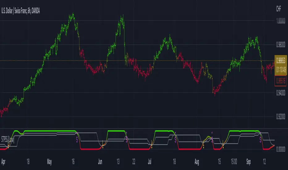
The Z-score is a low timeframe scalper which works best during choppy/ranging phases. The direction you should trade is determined by the last trend change. E.g. when the last trend change was from bearish market to bullish market and you are now in a choppy/ranging phase confirmed by e.g. Chop Zone or KAMA slope you want to do long trades.
Interpretation
The Z-score indicator is a momentum indicator which shows the number of standard deviations by which the value of a raw score (price/source) is above or below the mean value of what is being observed or measured. Easily explained, it is almost the same as Bollinger Bands with another visual representation form.
Signals
B -> Buy -> Z-score crosses above lower band
S -> Short -> Z-score crosses below upper band
BE -> Buy Exit -> Z-score crosses above 0
SE -> Sell Exit -> Z-score crosses below 0
If you were reading till here, thank you already. Now, follows a bunch of knowledge for people who don't know the concepts I talk about.
T3
The T3 moving average, short for "Tim Tillson's Triple Exponential Moving Average," is a technical indicator used in financial markets and technical analysis to smooth out price data over a specific period. It was developed by Tim Tillson, a software project manager at Hewlett-Packard, with expertise in Mathematics and Computer Science.
The T3 moving average is an enhancement of the traditional Exponential Moving Average (EMA) and aims to overcome some of its limitations. The primary goal of the T3 moving average is to provide a smoother representation of price trends while minimizing lag compared to other moving averages like Simple Moving Average (SMA), Weighted Moving Average (WMA), or EMA.
To compute the T3 moving average, it involves a triple smoothing process using exponential moving averages. Here's how it works:
Calculate the first exponential moving average (EMA1) of the price data over a specific period 'n.'
Calculate the second exponential moving average (EMA2) of EMA1 using the same period 'n.'
Calculate the third exponential moving average (EMA3) of EMA2 using the same period 'n.'
The formula for the T3 moving average is as follows:
T3 = 3 * (EMA1) - 3 * (EMA2) + (EMA3)
By applying this triple smoothing process, the T3 moving average is intended to offer reduced noise and improved responsiveness to price trends. It achieves this by incorporating multiple time frames of the exponential moving averages, resulting in a more accurate representation of the underlying price action.
JMA
The Jurik Moving Average (JMA) is a technical indicator used in trading to predict price direction. Developed by Mark Jurik, it’s a type of weighted moving average that gives more weight to recent market data rather than past historical data.
JMA is known for its superior noise elimination. It’s a causal, nonlinear, and adaptive filter, meaning it responds to changes in price action without introducing unnecessary lag. This makes JMA a world-class moving average that tracks and smooths price charts or any market-related time series with surprising agility.
In comparison to other moving averages, such as the Exponential Moving Average (EMA), JMA is known to track fast price movement more accurately. This allows traders to apply their strategies to a more accurate picture of price action.
Inverse Fisher Transform
The Inverse Fisher Transform is a transform used in DSP to alter the Probability Distribution Function (PDF) of a signal or in our case of indicators.
The result of using the Inverse Fisher Transform is that the output has a very high probability of being either +1 or –1. This bipolar probability distribution makes the Inverse Fisher Transform ideal for generating an indicator that provides clear buy and sell signals.
Hann Window
The Hann function (aka Hann Window) is named after the Austrian meteorologist Julius von Hann. It is a window function used to perform Hann smoothing.
Super Smoother
The Super Smoother uses a special mathematical process for the smoothing of data points.
The Super Smoother is a technical analysis indicator designed to be smoother and with less lag than a traditional moving average.
Adaptive Length
Length based on the dominant cycle length measured by a "dominant cycle measurement" algorithm.
Happy Trading!
Best regards,
simwai
---
Credits to
@cheatcountry
@everget
@loxx
@DasanC
@blackcat1402
Ehlers

Goertzel Adaptive JMA T3Hello Fellas,
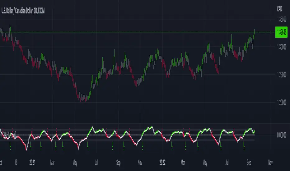
The Goertzel Adaptive JMA T3 is a powerful indicator that combines my own created Goertzel adaptive length with Jurik and T3 Moving Averages. The primary intention of the indicator is to demonstrate the new adaptive length algorithm by applying it on bleeding-edge MAs.
It is useable like any moving average, and the new Goertzel adaptive length algorithm can be used to make own indicators Goertzel adaptive.
Used Adaptive Length Algorithms
Normalized Goertzel Power: This uses the normalized power of the Goertzel algorithm to compute an adaptive length without the special operations, like detrending, Ehlers uses for his DFT adaptive length.
Ehlers Mod: This uses the Goertzel algorithm instead of the DFT, originally used by Ehlers, to compute a modified version of his original approach, which sticks as close as possible to the original approach.
Scoring System
The scoring system determines if bars are red or green and collects them.
Then, it goes through all collected red and green bars and checks how big they are and if they are above or below the selected MA. It is positive when green bars are under MA or when red bars are above MA.
Then, it accumulates the size for all positive green bars and for all positive red bars. The same happens for negative green and red bars.
Finally, it calculates the score by ((positiveGreenBars + positiveRedBars) / (negativeGreenBars + negativeRedBars)) * 100 with the scale 0–100.
Signals
Is the price above MA? -> bullish market
Is the price below MA? -> bearish market
Usage
Adjust the settings to reach the highest score, and enjoy an outstanding adaptive MA.
It should be useable on all timeframes. It is recommended to use the indicator on the timeframe where you can get the highest score.
Now, follows a bunch of knowledge for people who don't know about the concepts used here.
T3
The T3 moving average, short for "Tim Tillson's Triple Exponential Moving Average," is a technical indicator used in financial markets and technical analysis to smooth out price data over a specific period. It was developed by Tim Tillson, a software project manager at Hewlett-Packard, with expertise in Mathematics and Computer Science.
The T3 moving average is an enhancement of the traditional Exponential Moving Average (EMA) and aims to overcome some of its limitations. The primary goal of the T3 moving average is to provide a smoother representation of price trends while minimizing lag compared to other moving averages like Simple Moving Average (SMA), Weighted Moving Average (WMA), or EMA.
To compute the T3 moving average, it involves a triple smoothing process using exponential moving averages. Here's how it works:
Calculate the first exponential moving average (EMA1) of the price data over a specific period 'n.'
Calculate the second exponential moving average (EMA2) of EMA1 using the same period 'n.'
Calculate the third exponential moving average (EMA3) of EMA2 using the same period 'n.'
The formula for the T3 moving average is as follows:
T3 = 3 * (EMA1) - 3 * (EMA2) + (EMA3)
By applying this triple smoothing process, the T3 moving average is intended to offer reduced noise and improved responsiveness to price trends. It achieves this by incorporating multiple time frames of the exponential moving averages, resulting in a more accurate representation of the underlying price action.
JMA
The Jurik Moving Average (JMA) is a technical indicator used in trading to predict price direction. Developed by Mark Jurik, it’s a type of weighted moving average that gives more weight to recent market data rather than past historical data.
JMA is known for its superior noise elimination. It’s a causal, nonlinear, and adaptive filter, meaning it responds to changes in price action without introducing unnecessary lag. This makes JMA a world-class moving average that tracks and smooths price charts or any market-related time series with surprising agility.
In comparison to other moving averages, such as the Exponential Moving Average (EMA), JMA is known to track fast price movement more accurately. This allows traders to apply their strategies to a more accurate picture of price action.
Goertzel Algorithm
The Goertzel algorithm is a technique in digital signal processing (DSP) for efficient evaluation of individual terms of the Discrete Fourier Transform (DFT). It's particularly useful when you need to compute a small number of selected frequency components. Unlike direct DFT calculations, the Goertzel algorithm applies a single real-valued coefficient at each iteration, using real-valued arithmetic for real-valued input sequences. This makes it more numerically efficient when computing a small number of selected frequency components¹.
Discrete Fourier Transform
The Discrete Fourier Transform (DFT) is a mathematical technique used in signal processing to convert a finite sequence of equally-spaced samples of a function into a same-length sequence of equally-spaced samples of the discrete-time Fourier transform (DTFT), which is a complex-valued function of frequency . The DFT provides a frequency domain representation of the original input sequence .
Usage of DFT/Goertzel In Adaptive Length Algorithms
Adaptive length algorithms are automated trading systems that can dynamically adjust their parameters in response to real-time market data. This adaptability enables them to optimize their trading strategies as market conditions fluctuate. Both the Goertzel algorithm and DFT can be used in these algorithms to analyze market data and detect cycles or patterns, which can then be used to adjust the parameters of the trading strategy.
The Goertzel algorithm is more efficient than the DFT when you need to compute a small number of selected frequency components. However, for covering a full spectrum, the Goertzel algorithm has a higher order of complexity than fast Fourier transform (FFT) algorithms.
I hope this can help you somehow.
Thanks for reading, and keep it up.
Best regards,
simwai
---
Credits to:
@ClassicScott
@yatrader2
@cheatcountry
@loxx

FVG Detector [TradingFinder] Fair Value Gap-Imbalance-Mitigated🔵 Introduction
When the market makes a strong move in the form of a "Marubozu" or "Spike" candlestick and consecutive candles move without a retracement, the maximum place where a "FVG" or "Fair Value Gap" is created.
🔵 Definition
To describe this precisely, whenever a move occurs where the current candle does not cover the body of the previous and subsequent candles, a fair value gap is created.
Important : The significant point is that, because there is no equilibrium between buyers and sellers in these conditions, and market power is in the hands of buyers or sellers, the market is likely to move towards these areas.
An example of "FVG" in a price increase where we expect buying on the return to it.
An example of "FVG" in a downward trend where the market will move towards it in a downward direction.
🔵 How to Use
🟣 Bearish FVG
In a downward trend, "orange boxes" are drawn, which are the same and can act as "support" zones along the downward path, and we expect the price to continue its downward trend on return.
🟣 Bullish FVG
In an upward trend, "green boxes" are drawn, which are . They act exactly like support in the upward path, and we expect the price to continue its upward trend on return.
🟣 Auxiliary Definitions
Imbalance : As mentioned above, market power is in the hands of one of the two sides, buyers or sellers, and a non-equilibrium zone is created. It may be completed in whole or in part in subsequent price movements.
Mitigated : If the price returns to the "FVG" area and fills it, we call it "Mitigated," and most "pending" or "profit and loss limits" positions are executed. We will not have a specific reaction on the return of the price.
🔵 Settings
Very Aggressive : In addition to the initial condition, another condition is added. For an upward FVG, the maximum price of the last candle should be larger than the middle candle's maximum price. Similarly, for a downward FVG, the minimum price of the last candle should be smaller than the middle candle's minimum price. In this mode, a very small number of FVGs are eliminated.
Aggressive : In addition to the conditions of the Very Aggressive mode, in this mode, the size of the middle candle should not be small. In this mode, a larger number of FVGs are eliminated.
Defensive : In addition to the conditions of the Very Aggressive mode, in this mode, the size of the middle candle should be relatively large, and the majority of it should be made up of the body. Additionally, to identify upward FVGs, the second and third candles must be positive, and to identify downward FVGs, the second and third candles must be negative. In this mode, a large number of FVGs are eliminated, leaving only those with suitable quality.
Very Defensive : In addition to the conditions of the Defensive mode, the first and third candles should not be very small-bodied doji candles. In this mode, the majority of FVGs are filtered out, leaving only the highest quality ones.
🔵 Features
Show Demand FVG : Displays demand-related boxes, which can be "off" and "on."
Show Supply FVG : Displays supply-related boxes along the path, and can be turned "off" and "on."
🔵 Indicator Advantages
In this indicator, I have implemented 4 types of "filters" that allow you to select one based on the trading symbol, timeframe, etc. From "Very Aggressive" to "Very Defensive" mode, it is possible to select.
In most indicators, all FVGs are displayed, and the chart becomes full of lines. But this unique feature allows the trader to manage the drawing of boxes.

Rocket RSI from John EhlersWhat is Rocket RSI
Welles Wilder's original description of the relative strength index (RSI) in his 1978 New Concepts In Technical Trading Systems specified a calculation period of 14 days. This requirement led him on a 40-year quest to find the right length of data for calculating indicators and trading strategy rules. Many technicians touched on RSI and explained its applications. In this study we will obtain a more flexible and easier to interpret formulation (of the indicator). We will also estimate the algorithm to properly handle a statistical approach to technical analysis. Start with RSI Here is the original definition of the RSI indicator:
RSI = 100 - 100 / (1 + RS)
RS = Average gain from downtime over the specified time period / Average loss from downtime over the specified time period My first observation is that the factor of 100 is insignificant. Second, there is no need for averages because we take the ratio of closes (CU) to closes (CD) and if we accumulate the wins and losses independently, the averages emerge. Therefore We will only accumulate CU and CD. He can then write the RSI equation as:
RSI = 1 – 1 / (1 + CU / CD)
If he use a little algebra to put everything on a common denominator on the right side of the equation, the indicator equation becomes:
RSI = CU / (CU + CD)
In this formulation, if CU accumulation is zero, the RSI value is zero, and if CD accumulation is zero, the RSI value is 1. If you reduce the price action to its primitive level as a sine wave, it is easy to see that this RSI only has CU going from valley to peak and only CD going from peak to valley. This RSI follows the shape of the sine wave between these two limits. However, the sine wave oscillates between -1 and +1, not between 0 and +1. If we multiply the above equation by 2 and then subtract 1, we can make the RSI have the same swing limits as the sine wave. the product is as follows:
RSI = 2*CU / (CU + CD) – 1
Again, using a little algebra to put the right-hand side of the equation on a common denominator, the equation develops like this:
MyRSI = (CU – CD) / (CU + CD)
Again, the vertical scale of the RocketRSI indicator is in standard deviations. For example, -2 means it is two standard deviations below the mean. Since exceeding two standard deviations in the Gaussian probability distribution occurs in only 2.4% of the results
Because we are using the momentum of the dominant cycle period, the spike where the indicator falls below -2 provides a surgically precise timing signal to enter a long position. Similarly, exceeding the +2 standard deviation level is a timing signal to exit a long position or return to a short position. Therefore using the RocketRSI indicator is relatively intuitive. The only concern is whether a dominant cycle is present in the data, setting the indicator to half the dominant cycle period, and whether smoothing causes lag.
DETERMINING CYCLICAL TURNING POINTS
When you insert the chart you see an example of what the RocketRSI indicator looks like. Here you see that RocketRSI precisely displays cyclical turning points as statistical events. Cator can be applied. I used RS Length 10 because according to Ehlers, stocks and stock indexes usually have a more or less monthly cycle (about 20 bars). A cursory examination of Figure 2 shows that negative increases in the indicator correspond to excellent buying opportunities, while positive increases correspond to excellent selling opportunities. Exceeding +/- 2 on the indicator scale indicates that a cyclical reversal is a high probability event.

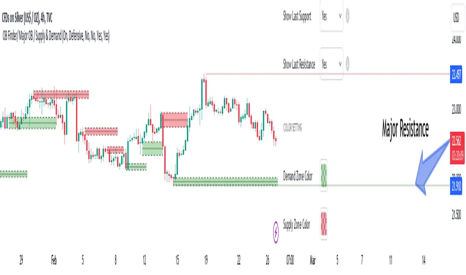
Order Blocks Finder [TradingFinder] Major OB | Supply and Demand🔵 Introduction
Drawing all order blocks on the path, especially in range-bound or channeling markets, fills the chart with lines, making it confusing rather than providing the trader with the best entry and exit points.
🔵 Reason for Indicator Creation
For traders familiar with market structure and only need to know the main accumulation points (best entry or exit points), and primary order blocks that act as strong sources of power.
🟣 Important Note
All order blocks, both ascending and descending, are identified and displayed on the chart when the structure of "BOS" or "CHOCH" is broken, which can also be identified with "MSS."
🔵 How to Use
When the indicator is installed, it plots all order blocks (active order blocks) and continues until the price reaches them. This continuation happens in boxes to have a better view in the TradingView chart.
Green Range : Ascending order blocks where we expect a price increase in these areas.
Red Range : Descending order blocks where we expect a price decrease in these areas.
🔵 Settings
Order block refine setting : When Order block refine is off, the supply and demand zones are the entire length of the order block (Low to High) in their standard state and cannot be improved. If you turn on Order block refine, supply and demand zones will improve using the error correction algorithm.
Refine type setting : Improving order blocks using the error correction algorithm can be done in two ways: Defensive and Aggressive. In the Aggressive method, the largest possible range is considered for order blocks.
🟣 Important
The main advantage of the Aggressive method is minimizing the loss of stops, but due to the widening of the supply or demand zone, the reward-to-risk ratio decreases significantly. The Aggressive method is suitable for individuals who take high-risk trades.
In the Defensive method, the range of order blocks is minimized to their standard state. In this case, fewer stops are triggered, and the reward-to-risk ratio is maximized in its optimal state. It is recommended for individuals who trade with low risk.
Show high level setting : If you want to display major high levels, set show high level to Yes.
Show low level setting : If you want to display major low levels, set show low level to Yes.
🔵 How to Use
The general view of this indicator is as follows.
When the price approaches the range, wait for the price reaction to confirm it, such as a pin bar or divergence.
If the price passes with a strong candle (spike), especially after a long-range or at the beginning of sessions, a powerful event is happening, and it is outside the credibility level.
An Example of a Valid Zone
An Example of Breakout and Invalid Zone. (My suggestion is not to use pending orders, especially when the market is highly volatile or before and after news.)
After reaching this zone, expect the price to move by at least the minimum candle that confirmed it or a price ceiling or floor.
🟣 Important : These factors can be more accurately measured with other trend finder indicators provided.
🔵 Auxiliary Tools
There is much talk about not using trend lines, candlesticks, Fibonacci, etc., in the web space. However, our suggestion is to create and use tools that can help you profit from this market.
• Fibonacci Retracement
• Trading Sessions
• Candlesticks
🔵 Advantages
• Plotting main OBs without additional lines;
• Suitable for timeframes M1, M5, M15, H1, and H4;
• Effective in Tokyo, Sydney, and London sessions;
• Plotting the main ceiling and floor to help identify the trend.
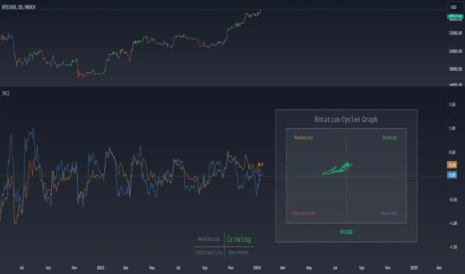
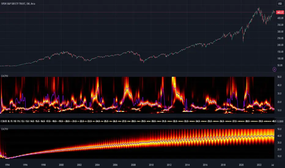
Rotation Cycles GraphRotation Cycles Graph Indicator
Overview:
The Rotation Cycles Graph Indicator is designed to visualize rotation cycles in financial markets. It aims to provide insights into shifts between various market phases, including growth, weakening, recovery, and contraction, allowing traders to potentially identify changing market dynamics.
Key Components:
Z-Score Calculation:
The indicator employs Z-score calculation to normalize data and identify deviations from the mean. This is instrumental in understanding the current state of the market relative to its historical behavior.
Ehlers Loop Visualization:
The Ehlers Loop function generates a visual representation of rotation cycles. It utilizes x and y coordinates on the chart to represent market conditions. These coordinates determine the position and categorization of the market state.
Table Visualization:
At the bottom of the chart, a table categorizes market conditions based on x and y values. This table serves as a reference to understand the current market phase.
Customizable Parameters:
The indicator offers users the flexibility to adjust several parameters:
Length and Smoothness: Users can set the length and smoothness parameters for the Z-score calculation, allowing for customization based on the market's volatility.
Graph Settings: Parameters such as bar scale, graph position, and the length of the tail for visualization can be fine-tuned to suit individual preferences.
Understanding Coordinates:
The x and y coordinates plotted on the chart represent specific market conditions. Interpretation of these coordinates aids in recognizing shifts in market behavior.
This screenshot shows visual representation behind logic of X and Y and their rotation cycles
Here is an example how rotation marker moved from growing to weakening and to the contraction quad, during a big market crush:
Note:
This indicator is a visualization tool and should be used in conjunction with other analytical methods for comprehensive market analysis.
Understanding the context and nuances of market dynamics is essential for accurate interpretation of the Rotation Cycles Graph Indicator.
Big thanks to @PineCodersTASC for their indicator, what I used as a reference
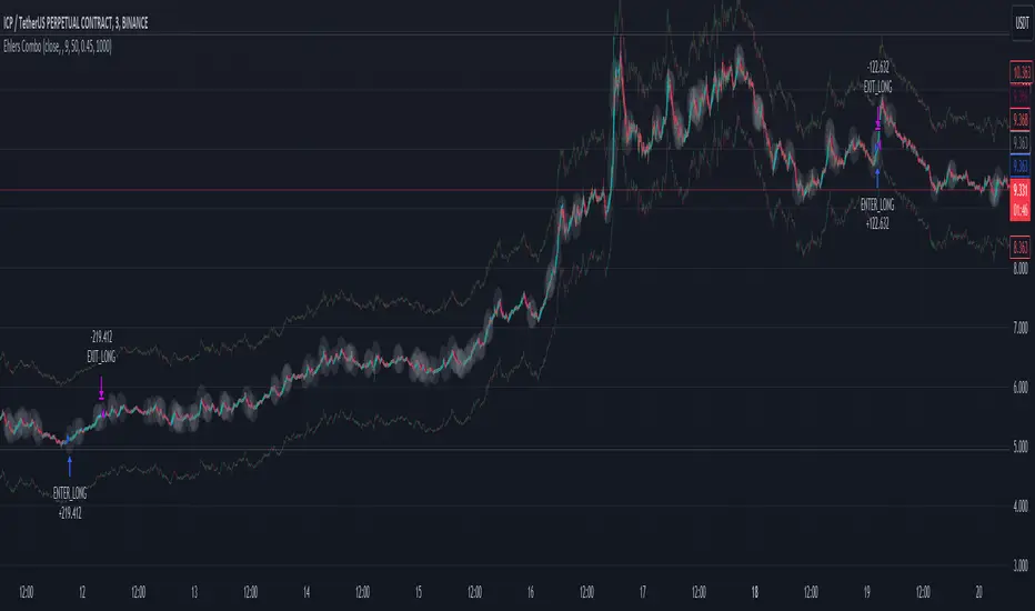
Ehlers Combo Strategy🚀 Presenting the Enhanced Ehlers Combo Strategy 🚀
Hello Traders! 👋 I'm thrilled to share the latest version of the Ehlers Combo Strategy v2.0. This powerful algorithm combines Ehlers Elegant Oscillator, Decycler, Instantaneous Trendline, Spearman Rank, and introduces the Signal to Noise Ratio for even more precise trading signals.
📊 Strategy Highlights:
Ehlers Elegant Oscillator: Captures market momentum and turning points.
Ehlers Decycler: Filters out market noise for clearer trend signals.
Instantaneous Trendline: Offers a dynamic view of the market trend.
Spearman Rank: Analyzes market rank correlations for enhanced insights.
Signal to Noise Ratio (SNR): Filters out noise for more accurate signals.
💡 Key Features & Customizations:
Adaptive Length: Enable adaptive length based on the market's current conditions.
SNR Threshold: Set your desired SNR threshold for filtering signals.
Exit Length: Define the length for exit signals.
📈 Trading Signals:
Long Entry: Elegant Oscillator and Decycler cross above 0, source crosses above Decycler, source is greater than an increasing Instantaneous Trendline, Spearman Rank is positive, and SNR exceeds the threshold.
Long Exit: Source crosses below the Instantaneous Trendline after entering a long position.
Short Entry: Elegant Oscillator and Decycler cross below 0, source crosses below Decycler, source is less than a decreasing Instantaneous Trendline, Spearman Rank is negative, and SNR exceeds the threshold.
Short Exit: Source crosses above the Instantaneous Trendline after entering a short position.
📊 Insights & Enhancements:
Dynamic Length: The strategy adapts its length dynamically based on market conditions.
Improved SNR: Signal to Noise Ratio ensures better filtering of signals.
Enhanced Visualization: The Elegant Oscillator now features improved color coding for a clearer interpretation.
🚨 Disclaimer:
Trading involves risk, and this script should be used judiciously. It's not a guaranteed profit machine, but with careful use, it can be a valuable addition to your toolkit.
Feel free to backtest, tweak, and make it your own! Let's conquer the markets together! 💪📈
🚀✨ Happy Trading! ✨🚀
---
🙌 Credits:
A big shoutout to the original contributors:
@blackcat1402
@cheatcountry
@DasanC
[Excalibur] Ehlers AutoCorrelation Periodogram ModifiedKeep your coins folks, I don't need them, don't want them. If you wish be generous, I do hope that charitable peoples worldwide with surplus food stocks may consider stocking local food banks before stuffing monetary bank vaults, for the crusade of remedying the needs of less than fortunate children, parents, elderly, homeless veterans, and everyone else who deserves nutritional sustenance for the soul.
DEDICATION:
This script is dedicated to the memory of Nikolai Dmitriyevich Kondratiev (Никола́й Дми́триевич Кондра́тьев) as tribute for being a pioneering economist and statistician, paving the way for modern econometrics by advocation of rigorous and empirical methodologies. One of his most substantial contributions to the study of business cycle theory include a revolutionary hypothesis recognizing the existence of dynamic cycle-like phenomenon inherent to economies that are characterized by distinct phases of expansion, stagnation, recession and recovery, what we now know as "Kondratiev Waves" (K-waves). Kondratiev was one of the first economists to recognize the vital significance of applying quantitative analysis on empirical data to evaluate economic dynamics by means of statistical methods. His understanding was that conceptual models alone were insufficient to adequately interpret real-world economic conditions, and that sophisticated analysis was necessary to better comprehend the nature of trending/cycling economic behaviors. Additionally, he recognized prosperous economic cycles were predominantly driven by a combination of technological innovations and infrastructure investments that resulted in profound implications for economic growth and development.
I will mention this... nation's economies MUST be supported and defended to continuously evolve incrementally in order to flourish in perpetuity OR suffer through eras with lasting ramifications of societal stagnation and implosion.
Analogous to the realm of economics, aperiodic cycles/frequencies, both enduring and ephemeral, do exist in all facets of life, every second of every day. To name a few that any blind man can naturally see are: heartbeat (cardiac cycles), respiration rates, circadian rhythms of sleep, powerful magnetic solar cycles, seasonal cycles, lunar cycles, weather patterns, vegetative growth cycles, and ocean waves. Do not pretend for one second that these basic aforementioned examples do not affect business cycle fluctuations in minuscule and monumental ways hour to hour, day to day, season to season, year to year, and decade to decade in every nation on the planet. Kondratiev's original seminal theories in macroeconomics from nearly a century ago have proven remarkably prescient with many of his antiquated elementary observations/notions/hypotheses in macroeconomics being scholastically studied and topically researched further. Therefore, I am compelled to honor and recognize his statistical insight and foresight.
If only.. Kondratiev could hold a pocket sized computer in the cup of both hands bearing the TradingView logo and platform services, I truly believe he would be amazed in marvelous delight with a GARGANTUAN smile on his face.
INTRODUCTION:
Firstly, this is NOT technically speaking an indicator like most others. I would describe it as an advanced cycle period detector to obtain market data spectral estimates with low latency and moderate frequency resolution. Developers can take advantage of this detector by creating scripts that utilize a "Dominant Cycle Source" input to adaptively govern algorithms. Be forewarned, I would only recommend this for advanced developers, not novice code dabbling. Although, there is some Pine wizardry introduced here for novice Pine enthusiasts to witness and learn from. AI did describe the code into one super-crunched sentence as, "a rare feat of exceptionally formatted code masterfully balancing visual clarity, precision, and complexity to provide immense educational value for both programming newcomers and expert Pine coders alike."
Understand all of the above aforementioned? Buckle up and proceed for a lengthy read of verbose complexity...
This is my enhanced and heavily modified version of autocorrelation periodogram (ACP) for Pine Script v5.0. It was originally devised by the mathemagician John Ehlers for detecting dominant cycles (frequencies) in an asset's price action. I have been sitting on code similar to this for a long time, but I decided to unleash the advanced code with my fashion. Originally Ehlers released this with multiple versions, one in a 2016 TASC article and the other in his last published 2013 book "Cycle Analytics for Traders", chapter 8. He wasn't joking about "concepts of advanced technical trading" and ACP is nowhere near to his most intimidating and ingenious calculations in code. I will say the book goes into many finer details about the original periodogram, so if you wish to delve into even more elaborate info regarding Ehlers' original ACP form AND how you may adapt algorithms, you'll have to obtain one. Note to reader, comparing Ehlers' original code to my chimeric code embracing the "Power of Pine", you will notice they have little resemblance.
What you see is a new species of autocorrelation periodogram combining Ehlers' innovation with my fascinations of what ACP could be in a Pine package. One other intention of this script's code is to pay homage to Ehlers' lifelong works. Like Kondratiev, Ehlers is also a hardcore cycle enthusiast. I intend to carry on the fire Ehlers envisioned and I believe that is literally displayed here as a pleasant "fiery" example endowed with Pine. With that said, I tried to make the code as computationally efficient as possible, without going into dozens of more crazy lines of code to speed things up even more. There's also a few creative modifications I made by making alterations to the originating formulas that I felt were improvements, one of them being lag reduction. By recently questioning every single thing I thought I knew about ACP, combined with the accumulation of my current knowledge base, this is the innovative revision I came up with. I could have improved it more but decided not to mind thrash too many TV members, maybe later...
I am now confident Pine should have adequate overhead left over to attach various indicators to the dominant cycle via input.source(). TV, I apologize in advance if in the future a server cluster combusts into a raging inferno... Coders, be fully prepared to build entire algorithms from pure raw code, because not all of the built-in Pine functions fully support dynamic periods (e.g. length=ANYTHING). Many of them do, as this was requested and granted a while ago, but some functions are just inherently finicky due to implementation combinations and MUST be emulated via raw code. I would imagine some comprehensive library or numerous authored scripts have portions of raw code for Pine built-ins some where on TV if you look diligently enough.
Notice: Unfortunately, I will not provide any integration support into member's projects at all. I have my own projects that require way too much of my day already. While I was refactoring my life (forgoing many other "important" endeavors) in the early half of 2023, I primarily focused on this code over and over in my surplus time. During that same time I was working on other innovations that are far above and beyond what this code is. I hope you understand.
The best way programmatically may be to incorporate this code into your private Pine project directly, after brutal testing of course, but that may be too challenging for many in early development. Being able to see the periodogram is also beneficial, so input sourcing may be the "better" avenue to tether portions of the dominant cycle to algorithms. Unique indication being able to utilize the dominantCycle may be advantageous when tethering this script to those algorithms. The easiest way is to manually set your indicators to what ACP recognizes as the dominant cycle, but that's actually not considered dynamic real time adaption of an indicator. Different indicators may need a proportion of the dominantCycle, say half it's value, while others may need the full value of it. That's up to you to figure that out in practice. Sourcing one or more custom indicators dynamically to one detector's dominantCycle may require code like this: `int sourceDC = int(math.max(6, math.min(49, input.source(close, "Dominant Cycle Source"))))`. Keep in mind, some algos can use a float, while algos with a for loop require an integer.
I have witnessed a few attempts by talented TV members for a Pine based autocorrelation periodogram, but not in this caliber. Trust me, coding ACP is no ordinary task to accomplish in Pine and modifying it blessed with applicable improvements is even more challenging. For over 4 years, I have been slowly improving this code here and there randomly. It is beautiful just like a real flame, but... this one can still burn you! My mind was fried to charcoal black a few times wrestling with it in the distant past. My very first attempt at translating ACP was a month long endeavor because PSv3 simply didn't have arrays back then. Anyways, this is ACP with a newer engine, I hope you enjoy it. Any TV subscriber can utilize this code as they please. If you are capable of sufficiently using it properly, please use it wisely with intended good will. That is all I beg of you.
Lastly, you now see how I have rasterized my Pine with Ehlers' swami-like tech. Yep, this whole time I have been using hline() since PSv3, not plot(). Evidently, plot() still has a deficiency limited to only 32 plots when it comes to creating intense eye candy indicators, the last I checked. The use of hline() is the optimal choice for rasterizing Ehlers styled heatmaps. This does only contain two color schemes of the many I have formerly created, but that's all that is essentially needed for this gizmo. Anything else is generally for a spectacle or seeing how brutal Pine can be color treated. The real hurdle is being able to manipulate colors dynamically with Merlin like capabilities from multiple algo results. That's the true challenging part of these heatmap contraptions to obtain multi-colored "predator vision" level indication. You now have basic hline() food for thought empowerment to wield as you can imaginatively dream in Pine projects.
PERIODOGRAM UTILITY IN REAL WORLD SCENARIOS:
This code is a testament to the abilities that have yet to be fully realized with indication advancements. Periodograms, spectrograms, and heatmaps are a powerful tool with real-world applications in various fields such as financial markets, electrical engineering, astronomy, seismology, and neuro/medical applications. For instance, among these diverse fields, it may help traders and investors identify market cycles/periodicities in financial markets, support engineers in optimizing electrical or acoustic systems, aid astronomers in understanding celestial object attributes, assist seismologists with predicting earthquake risks, help medical researchers with neurological disorder identification, and detection of asymptomatic cardiovascular clotting in the vaxxed via full body thermography. In either field of study, technologies in likeness to periodograms may very well provide us with a better sliver of analysis beyond what was ever formerly invented. Periodograms can identify dominant cycles and frequency components in data, which may provide valuable insights and possibly provide better-informed decisions. By utilizing periodograms within aspects of market analytics, individuals and organizations can potentially refrain from making blinded decisions and leverage data-driven insights instead.
PERIODOGRAM INTERPRETATION:
The periodogram renders the power spectrum of a signal, with the y-axis representing the periodicity (frequencies/wavelengths) and the x-axis representing time. The y-axis is divided into periods, with each elevation representing a period. In this periodogram, the y-axis ranges from 6 at the very bottom to 49 at the top, with intermediate values in between, all indicating the power of the corresponding frequency component by color. The higher the position occurs on the y-axis, the longer the period or lower the frequency. The x-axis of the periodogram represents time and is divided into equal intervals, with each vertical column on the axis corresponding to the time interval when the signal was measured. The most recent values/colors are on the right side.
The intensity of the colors on the periodogram indicate the power level of the corresponding frequency or period. The fire color scheme is distinctly like the heat intensity from any casual flame witnessed in a small fire from a lighter, match, or camp fire. The most intense power would be indicated by the brightest of yellow, while the lowest power would be indicated by the darkest shade of red or just black. By analyzing the pattern of colors across different periods, one may gain insights into the dominant frequency components of the signal and visually identify recurring cycles/patterns of periodicity.
SETTINGS CONFIGURATIONS BRIEFLY EXPLAINED:
Source Options: These settings allow you to choose the data source for the analysis. Using the `Source` selection, you may tether to additional data streams (e.g. close, hlcc4, hl2), which also may include samples from any other indicator. For example, this could be my "Chirped Sine Wave Generator" script found in my member profile. By using the `SineWave` selection, you may analyze a theoretical sinusoidal wave with a user-defined period, something already incorporated into the code. The `SineWave` will be displayed over top of the periodogram.
Roofing Filter Options: These inputs control the range of the passband for ACP to analyze. Ehlers had two versions of his highpass filters for his releases, so I included an option for you to see the obvious difference when performing a comparison of both. You may choose between 1st and 2nd order high-pass filters.
Spectral Controls: These settings control the core functionality of the spectral analysis results. You can adjust the autocorrelation lag, adjust the level of smoothing for Fourier coefficients, and control the contrast/behavior of the heatmap displaying the power spectra. I provided two color schemes by checking or unchecking a checkbox.
Dominant Cycle Options: These settings allow you to customize the various types of dominant cycle values. You can choose between floating-point and integer values, and select the rounding method used to derive the final dominantCycle values. Also, you may control the level of smoothing applied to the dominant cycle values.
DOMINANT CYCLE VALUE SELECTIONS:
External to the acs() function, the code takes a dominant cycle value returned from acs() and changes its numeric form based on a specified type and form chosen within the indicator settings. The dominant cycle value can be represented as an integer or a decimal number, depending on the attached algorithm's requirements. For example, FIR filters will require an integer while many IIR filters can use a float. The float forms can be either rounded, smoothed, or floored. If the resulting value is desired to be an integer, it can be rounded up/down or just be in an integer form, depending on how your algorithm may utilize it.
AUTOCORRELATION SPECTRUM FUNCTION BASICALLY EXPLAINED:
In the beginning of the acs() code, the population of caches for precalculated angular frequency factors and smoothing coefficients occur. By precalculating these factors/coefs only once and then storing them in an array, the indicator can save time and computational resources when performing subsequent calculations that require them later.
In the following code block, the "Calculate AutoCorrelations" is calculated for each period within the passband width. The calculation involves numerous summations of values extracted from the roofing filter. Finally, a correlation values array is populated with the resulting values, which are normalized correlation coefficients.
Moving on to the next block of code, labeled "Decompose Fourier Components", Fourier decomposition is performed on the autocorrelation coefficients. It iterates this time through the applicable period range of 6 to 49, calculating the real and imaginary parts of the Fourier components. Frequencies 6 to 49 are the primary focus of interest for this periodogram. Using the precalculated angular frequency factors, the resulting real and imaginary parts are then utilized to calculate the spectral Fourier components, which are stored in an array for later use.
The next section of code smooths the noise ridden Fourier components between the periods of 6 and 49 with a selected filter. This species also employs numerous SuperSmoothers to condition noisy Fourier components. One of the big differences is Ehlers' versions used basic EMAs in this section of code. I decided to add SuperSmoothers.
The final sections of the acs() code determines the peak power component for normalization and then computes the dominant cycle period from the smoothed Fourier components. It first identifies a single spectral component with the highest power value and then assigns it as the peak power. Next, it normalizes the spectral components using the peak power value as a denominator. It then calculates the average dominant cycle period from the normalized spectral components using Ehlers' "Center of Gravity" calculation. Finally, the function returns the dominant cycle period along with the normalized spectral components for later external use to plot the periodogram.
POST SCRIPT:
Concluding, I have to acknowledge a newly found analyst for assistance that I couldn't receive from anywhere else. For one, Claude doesn't know much about Pine, is unfortunately color blind, and can't even see the Pine reference, but it was able to intuitively shred my code with laser precise realizations. Not only that, formulating and reformulating my description needed crucial finesse applied to it, and I couldn't have provided what you have read here without that artificial insight. Finding the right order of words to convey the complexity of ACP and the elaborate accompanying content was a daunting task. No code in my life has ever absorbed so much time and hard fricking work, than what you witness here, an ACP gem cut pristinely. I'm unveiling my version of ACP for an empowering cause, in the hopes a future global army of code wielders will tether it to highly functional computational contraptions they might possess. Here is ACP fully blessed poetically with the "Power of Pine" in sublime code. ENJOY!
Gaussian Fisher Transform Price Reversals - FTRHello Traders !
Looking for better trading results ?
"This indicator shows you how to identify price reversals in a timely manner." John F. Ehlers
Introduction :
The Gaussian Fisher Transform Price Reversals indicator, dubbed FTR for short, is a stat based price reversal detection indicator inspired by and based on the work of the electrical engineer now private trader John F. Ehlers.
The Fisher Transform :
It is a common assumption that prices have a gaussian / normal probability density function(PDF), i.e. a sample of n close prices would be normally distributed if the probability of observing a price value say at any given standard deviation range is equal to that probability in the case of the normal distribution, e.g. 68% off all samples fell within one standard deviation around the mean, which is what we would expect if the data was normal.
However Price Action is not normally distributed and thus can not be conventionally interpreted in this way, Formally the Fisher Transform, transforms the distribution of bounded ranging price action (were price action takes values in a range from -1 to 1) into that of a normal distribution, alternatively it may be said the Fisher Transform changes the PDF of any waveform so that the transformed output has n approximately Gaussian PDF, It does so through the following equations. taken directly from the work of John F. Ehlers - Using The Fisher Transform
By substituting price data in the above formulas, bounded ranging price actions (over a given user defined period lookback - this determines the range price ranges in, see the Intermediate formula above) distribution is transformed to that in the normal case. This means when the input, the Intermediate ,(the Midpoint - see formula above) approaches either limit within the range the outputs are greatly amplified, this amplification accentuates /puts more weight on the larger deviations or limits within the range, conversely when price action is varying round the mean of the range the output is approximately equal to unity (the input is approximately equal to the input, the intermediate)
The inputs (Intermediates) are converted to normal outputs and the nonlinear Transfer of the Fisher Transform with varying senesitivity's (gammas) can be seen in the graph / image above. Although sensitivity adjustments are not currently available in this script (I forgot to add it) the outputs may be greatly amplified as gamma (the coefficient of the Fisher Transformation - see Fish equation) approaches 1. the purple line show this graphically, as a higher gamma leads to a greater amplification than in the standard case (the red line which is the standard fisher transformation, the black plot is the Fish with a gamma of 1, which is unity sensativity)
Reversal plots and Breakouts :
- Support lines are plotted with their corresponding Fish value when there is a crossover of the Fish and Fish SMA <= a given standard deviation of Fish
- Resistance lines are plotted with their corresponding Fish value when there is a crossunder of the Fish and Fish SMA >= a given standard deviation of Fish
- Reversals are these support and resistance line plots
Breakouts and Volume bars :
Breakouts cause the reversal lines to break (when the high/low is above the resistance/support), Breakouts are more "high quality" when they occur conditional on high volume, the highlighted bars represent volume standard deviations ranging from -3 to 3. When breakouts occure on high volume this may be a sign of the continutaion of the trend (reversals would signify the start of a new trend).
Hope you enjoy, Happy Trading !
(be sure to rocket the script if you liked it, this helps me know which of my scripts are the most useful)

TASC 2023.04 Undersampled Double MA█ OVERVIEW
TASC's April 2023 edition of Traders' Tips features an article entitled "Just Ignore Them: Undersampling The Data As A Smoothing Technique" by John Ehlers, which explores a method for reducing noise through data sampling. This script implements the article's proposed Undersampled Double MA indicator.
█ CONCEPTS
The conventional approach to reducing the impact of noise in the market data on trading rules is to use smoothing filters like moving averages. However, John Ehlers suggests that changing the sample rate of the datastream is a simple and effective way to smooth the data and reduce noise. Specifically, he argues that undersampling the data removes high-frequency components contributing to noisiness. Notably, the elimination of these components produces less lag than that of conventional smoothing filters.
The Undersampled Double MA indicator implemented in this script represents a practical application of smoothing with undersampling. It samples the data at a given rate (for instance, once every five bars, as suggested by Ehlers), then processes the resulting data using a Hann window filter with two different periods, producing two smooth data streams that traders can use in the same way as the combination of two conventional moving averages of different lengths (i.e., fast and slow MAs).
█ CALCULATIONS
The script samples data once every N th bar (by default, N = 5) and smooths the undersampled data with 6-period and 12-period Hann filters, which it plots on the main chart. Users can adjust the sampling period and the periods of each Hann filter to their liking from the inputs in the script settings.
TASC 2023.03 Every Little Bit Helps - Special EditionMy first Published contribution.
Gracious thank you to all Pine Coders,
this has subtle features that have multiple shifts based on inputs.
with some experimentation, one might try pushing other sources
at the hue dials and see more dynamic indication.
for John Ehlers article
TASC Magazine This Month.
- Special Edition.
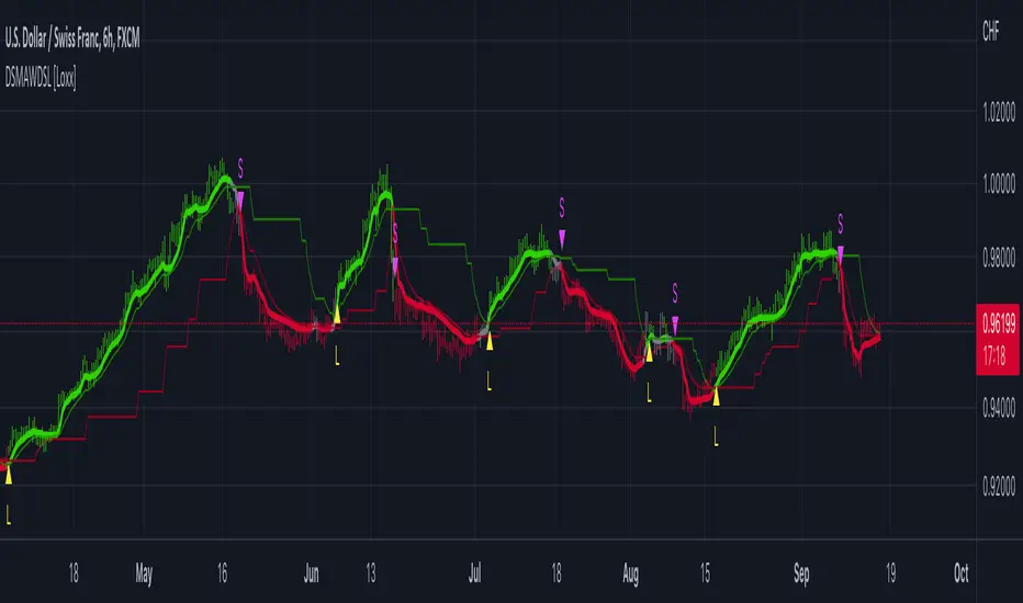
PA-Adaptive T3 Loxxer [Loxx]PA-Adaptive T3 Loxxer is a Loxxer indicator that is Phase Accumulation Cycle adaptive and uses T3 moving average for smoothing instead of the typical SMA or EMA . this allows for smoother signals by reducing noise.
What is Loxxer?
The Loxxer indicator is a technical analysis tool that compares the most recent maximum and minimum prices to the previous period's equivalent price to measure the demand of the underlying asset.
What is the Phase Accumulation Cycle?
The phase accumulation method of computing the dominant cycle is perhaps the easiest to comprehend. In this technique, we measure the phase at each sample by taking the arctangent of the ratio of the quadrature component to the in-phase component. A delta phase is generated by taking the difference of the phase between successive samples. At each sample we can then look backwards, adding up the delta phases.When the sum of the delta phases reaches 360 degrees, we must have passed through one full cycle, on average.The process is repeated for each new sample.
The phase accumulation method of cycle measurement always uses one full cycle’s worth of historical data.This is both an advantage and a disadvantage.The advantage is the lag in obtaining the answer scales directly with the cycle period.That is, the measurement of a short cycle period has less lag than the measurement of a longer cycle period. However, the number of samples used in making the measurement means the averaging period is variable with cycle period. longer averaging reduces the noise level compared to the signal.Therefore, shorter cycle periods necessarily have a higher out- put signal-to-noise ratio.
Included
Bar coloring
Signals
Alerts
Loxx's Expanded Source Types
Divergences

TASC 2023.03 Every Little Bit Helps█ OVERVIEW
TASC's February 2023 edition of Traders' Tips includes an article titled "Every Little Bit Helps: Averaging The Open And Close To Reduce Noise" by John Ehlers. This code implements the numerical example from this article.
█ CONCEPTS
Using theories from digital signal processing as a starting point, John Ehlers argues that using the average of the open and close as the source time series of an indicator instead of using only the closing price can often lead to noise reduction in the output. This effect especially applies when there is no gap between the current bar's opening and the previous bar's closing prices. This trick can reduce noise in many common indicators such as the RSI, MACD, and Stochastic.
█ CALCULATIONS
Following the example presented in the original publication, this script illustrates the proposed strategy using the Relative Strength Index (RSI) as a test indicator. It plots two series:
RSI calculated using only closing prices as its source.
RSI of the same length as the first, but calculated using the average of open and close prices as its source, i.e. (open+close)/2 .
This script demonstrates that using the average of open and close as the calculation source results in a smoother indicator. To visually emphasize the advantage of this proposed trick, the script's color scheme is sensitive to both the RSI value and the difference between the two RSI data streams.
inverse_fisher_transform_adaptive_stochastic█ Description
The indicator is the implementation of inverse fisher transform an indicator transform of the adaptive stochastic (dominant cycle), as in the Cycle Analytics for Trader pg. 198 (John F. Ehlers). Indicator transformation in brief means reshaping the indicator to be more interpretable. The inverse fisher transform is achieved by compressing values near the extremes many extraneous and irrelevant wiggles are removed from the indicator, as cited.
█ Inverse Fisher Transform
input = 2*(adaptive_stoc - .5)
output = e(2*k*input) -1 / e(2*k*input) +1
█ Feature:
iFish i.e. output value
trigger i.e. previous 1 bar of iFish * 0.90
if iFish crosses above the trigger, consider a buy indicated with the green line
while, iFish crosses below the trigger, consider a sell indicate by the red line
in addition iFish needs to be greater than the previous iFish

convolution
Description:
Convolution indicators aim to identify a major reversal in the price direction so that one can trade the market primarily in the direction of the ensuing trend, as described in the Cycle Analytics for Traders, by John F. Ehlers pg. 165. The notion is based on the concept of the two price segments are perfectly correlated (cross-correlated) that have been folded at the horizontal point, since high correlation exists only at the market turning point, e.g. price decreases linearly until the bottom is reached and then increases linearly after the bottom occurs and vice versa. The vertical scale is the lookback period, while the value is converted to colors.
Features:
High-pass filter and Smoothing function on the input data
Major reversals are identified by plumes pointing backward to the time of the price reversal
Bullish reversal identified by the green color of the indicator,
while Bearish reversal identified by a red color dominated the indicator

swami_rsi
Description:
As in the practices, most traders find it hard to set the proper lookback period of the indicator to be used. SwamiCharts offers a comprehensive way to visualize the indicator used over a range of lookback periods. The SwamiCharts of Relative Strength Index (RSI), was developed by Ehlers - see Cycle Analytics for Traders, chapter 16. The indicator was computed over multiple times of the range of lookback period for the Relative Strength Index (RSI), from the deficient period to the relatively high lookback period i.e. 1 to 48, then plotted as one heatmap.
Features:
In this indicator, the improvement is to utilize the color(dot)rgb() function, which finds to giving a relatively lower time to compute, and follows the original color scheme.
The confirmation level, which assumed of 25

TASC 2022.11 Phasor Analysis█ OVERVIEW
TASC's November 2022 edition Traders' Tips includes an article by John Ehlers titled "Recurring Phase Of Cycle Analysis". This is the code that implements the phasor analysis indicator presented in this publication.
█ CONCEPTS
The article explores the use of phasor analysis to identify market trends.
An ordinary rotating phasor diagram is a two-dimensional vector, anchored to the origin, whose rotation rate corresponds to the cycle period in the price data stream. Similarly, Ehlers' phasor is a representation of angular phase rotation along the course of time. Its angle reflects the current phase of the cycle. Angles -180, -90, +90 and +180 degrees correspond to the beginning, valley, peak and end of the cycle, respectively.
If the observed cycle is very long, the market can be considered trending . In his article, John Ehlers defined trending behavior to occur when the derived instantaneous cycle period value is greater that 60 bars. The author also introduced guidelines for long and short entries in a trending state. Depending on the tuning of the indicator period input, a long entry position may occur when the phasor angle is around the approximate vicinity of −90 degrees, while a short entry position may occur when the phasor angle will be around the approximate vicinity of +90 degrees. Applying these definitive guidelines, the author proposed a state variable that is indicated by +1 for a trending long position, 0 for cycling, and −1 for a trending short position (or out).
The phasor angle, the cycle period, and the state variable are made available with three selectable display modes provided for this TradingView indicator.
█ CALCULATIONS
The calculations are carried out as follows.
First, the price data stream is correlated with cosine and sine of a fixed cycle period. This produces two new data streams that correspond to the projections of the frequency domain phasor diagram to the horizontal (so-called real ) and vertical (so-called imaginary ) axis respectively. The wavelength of the cycle period input should be set for the midrange vicinities of the phasor to coincide with the peaks and valleys of the charted price data.
Secondly, the phase angle of the phasor is easily computed as the arctangent of the ratio of the imaginary component to the real component. The difference between the current phasor values and its last is then employed to calculate a derived instantaneous period and market state. This computation is then repeated successively for each individual bar over the entire duration of the data set.

Stochastic of Two-Pole SuperSmoother [Loxx]Stochastic of Two-Pole SuperSmoother is a Stochastic Indicator that takes as input Two-Pole SuperSmoother of price. Includes gradient coloring and Discontinued Signal Lines signals with alerts.
What is Ehlers ; Two-Pole Super Smoother?
From "Cycle Analytics for Traders Advanced Technical Trading Concepts" by John F. Ehlers
A SuperSmoother filter is used anytime a moving average of any type would otherwise be used, with the result that the SuperSmoother filter output would have substantially less lag for an equivalent amount of smoothing produced by the moving average. For example, a five-bar SMA has a cutoff period of approximately 10 bars and has two bars of lag. A SuperSmoother filter with a cutoff period of 10 bars has a lag a half bar larger than the two-pole modified Butterworth filter.Therefore, such a SuperSmoother filter has a maximum lag of approximately 1.5 bars and even less lag into the attenuation band of the filter. The differential in lag between moving average and SuperSmoother filter outputs becomes even larger when the cutoff periods are larger.
Market data contain noise, and removal of noise is the reason for using smoothing filters. In fact, market data contain several kinds of noise. I’ll group one kind of noise as systemic, caused by the random events of trades being exercised. A second kind of noise is aliasing noise, caused by the use of sampled data. Aliasing noise is the dominant term in the data for shorter cycle periods.
It is easy to think of market data as being a continuous waveform, but it is not. Using the closing price as representative for that bar constitutes one sample point. It doesn’t matter if you are using an average of the high and low instead of the close, you are still getting one sample per bar. Since sampled data is being used, there are some dSP aspects that must be considered. For example, the shortest analysis period that is possible (without aliasing)2 is a two-bar cycle.This is called the Nyquist frequency, 0.5 cycles per sample.A perfect two-bar sine wave cycle sampled at the peaks becomes a square wave due to sampling. However, sampling at the cycle peaks can- not be guaranteed, and the interference between the sampling frequency and the data frequency creates the aliasing noise.The noise is reduced as the data period is longer. For example, a four-bar cycle means there are four samples per cycle. Because there are more samples, the sampled data are a better replica of the sine wave component. The replica is better yet for an eight-bar data component.The improved fidelity of the sampled data means the aliasing noise is reduced at longer and longer cycle periods.The rate of reduction is 6 dB per octave. My experience is that the systemic noise rarely is more than 10 dB below the level of cyclic information, so that we create two conditions for effective smoothing of aliasing noise:
1. It is difficult to use cycle periods shorter that two octaves below the Nyquist frequency.That is, an eight-bar cycle component has a quantization noise level 12 dB below the noise level at the Nyquist frequency. longer cycle components therefore have a systemic noise level that exceeds the aliasing noise level.
2. A smoothing filter should have sufficient selectivity to reduce aliasing noise below the systemic noise level. Since aliasing noise increases at the rate of 6 dB per octave above a selected filter cutoff frequency and since the SuperSmoother attenuation rate is 12 dB per octave, the Super- Smoother filter is an effective tool to virtually eliminate aliasing noise in the output signal.
What are DSL Discontinued Signal Line?
A lot of indicators are using signal lines in order to determine the trend (or some desired state of the indicator) easier. The idea of the signal line is easy : comparing the value to it's smoothed (slightly lagging) state, the idea of current momentum/state is made.
Discontinued signal line is inheriting that simple signal line idea and it is extending it : instead of having one signal line, more lines depending on the current value of the indicator.
"Signal" line is calculated the following way :
When a certain level is crossed into the desired direction, the EMA of that value is calculated for the desired signal line
When that level is crossed into the opposite direction, the previous "signal" line value is simply "inherited" and it becomes a kind of a level
This way it becomes a combination of signal lines and levels that are trying to combine both the good from both methods.
In simple terms, DSL uses the concept of a signal line and betters it by inheriting the previous signal line's value & makes it a level.
Included:
Bar coloring
Alerts
Signals
Loxx's Expanded Source Types
Adaptive Two-Pole Super Smoother Entropy MACD [Loxx]Adaptive Two-Pole Super Smoother Entropy (Math) MACD is an Ehlers Two-Pole Super Smoother that is transformed into an MACD oscillator using entropy mathematics. Signals are generated using Discontinued Signal Lines.
What is Ehlers; Two-Pole Super Smoother?
From "Cycle Analytics for Traders Advanced Technical Trading Concepts" by John F. Ehlers
A SuperSmoother filter is used anytime a moving average of any type would otherwise be used, with the result that the SuperSmoother filter output would have substantially less lag for an equivalent amount of smoothing produced by the moving average. For example, a five-bar SMA has a cutoff period of approximately 10 bars and has two bars of lag. A SuperSmoother filter with a cutoff period of 10 bars has a lag a half bar larger than the two-pole modified Butterworth filter.Therefore, such a SuperSmoother filter has a maximum lag of approximately 1.5 bars and even less lag into the attenuation band of the filter. The differential in lag between moving average and SuperSmoother filter outputs becomes even larger when the cutoff periods are larger.
Market data contain noise, and removal of noise is the reason for using smoothing filters. In fact, market data contain several kinds of noise. I’ll group one kind of noise as systemic, caused by the random events of trades being exercised. A second kind of noise is aliasing noise, caused by the use of sampled data. Aliasing noise is the dominant term in the data for shorter cycle periods.
It is easy to think of market data as being a continuous waveform, but it is not. Using the closing price as representative for that bar constitutes one sample point. It doesn’t matter if you are using an average of the high and low instead of the close, you are still getting one sample per bar. Since sampled data is being used, there are some dSP aspects that must be considered. For example, the shortest analysis period that is possible (without aliasing)2 is a two-bar cycle.This is called the Nyquist frequency, 0.5 cycles per sample.A perfect two-bar sine wave cycle sampled at the peaks becomes a square wave due to sampling. However, sampling at the cycle peaks can- not be guaranteed, and the interference between the sampling frequency and the data frequency creates the aliasing noise.The noise is reduced as the data period is longer. For example, a four-bar cycle means there are four samples per cycle. Because there are more samples, the sampled data are a better replica of the sine wave component. The replica is better yet for an eight-bar data component.The improved fidelity of the sampled data means the aliasing noise is reduced at longer and longer cycle periods.The rate of reduction is 6 dB per octave. My experience is that the systemic noise rarely is more than 10 dB below the level of cyclic information, so that we create two conditions for effective smoothing of aliasing noise:
1. It is difficult to use cycle periods shorter that two octaves below the Nyquist frequency.That is, an eight-bar cycle component has a quantization noise level 12 dB below the noise level at the Nyquist frequency. longer cycle components therefore have a systemic noise level that exceeds the aliasing noise level.
2. A smoothing filter should have sufficient selectivity to reduce aliasing noise below the systemic noise level. Since aliasing noise increases at the rate of 6 dB per octave above a selected filter cutoff frequency and since the SuperSmoother attenuation rate is 12 dB per octave, the Super- Smoother filter is an effective tool to virtually eliminate aliasing noise in the output signal.
What are DSL Discontinued Signal Line?
A lot of indicators are using signal lines in order to determine the trend (or some desired state of the indicator) easier. The idea of the signal line is easy : comparing the value to it's smoothed (slightly lagging) state, the idea of current momentum/state is made.
Discontinued signal line is inheriting that simple signal line idea and it is extending it : instead of having one signal line, more lines depending on the current value of the indicator.
"Signal" line is calculated the following way :
When a certain level is crossed into the desired direction, the EMA of that value is calculated for the desired signal line
When that level is crossed into the opposite direction, the previous "signal" line value is simply "inherited" and it becomes a kind of a level
This way it becomes a combination of signal lines and levels that are trying to combine both the good from both methods.
In simple terms, DSL uses the concept of a signal line and betters it by inheriting the previous signal line's value & makes it a level.
Included:
Bar coloring
Alerts
Signals
Loxx's Expanded Source Types

FDI-Adaptive Fisher Transform [Loxx]FDI-Adaptive Fisher Transform is a Fractal Dimension Adaptive Fisher Transform indicator.
What is the Fractal Dimension Index?
The goal of the fractal dimension index is to determine whether the market is trending or in a trading range. It does not measure the direction of the trend. A value less than 1.5 indicates that the price series is persistent or that the market is trending. Lower values of the FDI indicate a stronger trend. A value greater than 1.5 indicates that the market is in a trading range and is acting in a more random fashion.
What is Fisher Transform?
The Fisher Transform is a technical indicator created by John F. Ehlers that converts prices into a Gaussian normal distribution.
The indicator highlights when prices have moved to an extreme, based on recent prices. This may help in spotting turning points in the price of an asset. It also helps show the trend and isolate the price waves within a trend.
Included:
Zero-line and signal cross options for bar coloring
Customizable overbought/oversold thresh-holds
Alerts
Signals
Deviation Scaled Moving Average w/ DSL [Loxx]Deviation Scaled Moving Average w/ DSL as described in the “The Deviation-Scaled Moving Average.” article of July 2018 TASC . This is an adaptive moving average average that has the ability to rapidly adapt to volatility in price movement. This version adds Discontinued Signal Lines create the buy/sell signals.
What are DSL Discontinued Signal Line?
A lot of indicators are using signal lines in order to determine the trend (or some desired state of the indicator) easier. The idea of the signal line is easy : comparing the value to it's smoothed (slightly lagging) state, the idea of current momentum/state is made.
Discontinued signal line is inheriting that simple signal line idea and it is extending it : instead of having one signal line, more lines depending on the current value of the indicator.
"Signal" line is calculated the following way :
When a certain level is crossed into the desired direction, the EMA of that value is calculated for the desired signal line
When that level is crossed into the opposite direction, the previous "signal" line value is simply "inherited" and it becomes a kind of a level
This way it becomes a combination of signal lines and levels that are trying to combine both the good from both methods.
In simple terms, DSL uses the concept of a signal line and betters it by inheriting the previous signal line's value & makes it a level.
Included
2 Signal types
Alerts
Loxx's Expanded Source Types
Bar coloring
STD/Clutter Filtered, One-Sided, N-Sinc-Kernel, EFIR Filt [Loxx]STD/Clutter Filtered, One-Sided, N-Sinc-Kernel, EFIR Filt is a normalized Cardinal Sine Filter Kernel Weighted Fir Filter that uses Ehler's FIR filter calculation instead of the general FIR filter calculation. This indicator has Kalman Velocity lag reduction, a standard deviation filter, a clutter filter, and a kernel noise filter. When calculating the Kernels, the both sides are calculated, then smoothed, then sliced to just the Right side of the Kernel weights. Lastly, blackman windowing is used for our purposes here. You can read about blackman windowing here:
Blackman window
Advantages of Blackman Window over Hamming Window Method for designing FIR Filter
The Kernel amplitudes are shown below with their corresponding values in yellow:
This indicator is intended to be used with Heikin-Ashi source inputs, specially HAB Median. You can read about this here:
Moving Average Filters Add-on w/ Expanded Source Types
What is a Finite Impulse Response Filter?
In signal processing, a finite impulse response (FIR) filter is a filter whose impulse response (or response to any finite length input) is of finite duration, because it settles to zero in finite time. This is in contrast to infinite impulse response (IIR) filters, which may have internal feedback and may continue to respond indefinitely (usually decaying).
The impulse response (that is, the output in response to a Kronecker delta input) of an Nth-order discrete-time FIR filter lasts exactly {\displaystyle N+1}N+1 samples (from first nonzero element through last nonzero element) before it then settles to zero.
FIR filters can be discrete-time or continuous-time, and digital or analog.
A FIR filter is (similar to, or) just a weighted moving average filter, where (unlike a typical equally weighted moving average filter) the weights of each delay tap are not constrained to be identical or even of the same sign. By changing various values in the array of weights (the impulse response, or time shifted and sampled version of the same), the frequency response of a FIR filter can be completely changed.
An FIR filter simply CONVOLVES the input time series (price data) with its IMPULSE RESPONSE. The impulse response is just a set of weights (or "coefficients") that multiply each data point. Then you just add up all the products and divide by the sum of the weights and that is it; e.g., for a 10-bar SMA you just add up 10 bars of price data (each multiplied by 1) and divide by 10. For a weighted-MA you add up the product of the price data with triangular-number weights and divide by the total weight.
Ultra Low Lag Moving Average's weights are designed to have MAXIMUM possible smoothing and MINIMUM possible lag compatible with as-flat-as-possible phase response.
Ehlers FIR Filter
Ehlers Filter (EF) was authored, not surprisingly, by John Ehlers. Read all about them here: Ehlers Filters
What is Normalized Cardinal Sine?
The sinc function sinc (x), also called the "sampling function," is a function that arises frequently in signal processing and the theory of Fourier transforms.
In mathematics, the historical unnormalized sinc function is defined for x ≠ 0 by
sinc x = sinx / x
In digital signal processing and information theory, the normalized sinc function is commonly defined for x ≠ 0 by
sinc x = sin(pi * x) / (pi * x)
What is a Clutter Filter?
For our purposes here, this is a filter that compares the slope of the trading filter output to a threshold to determine whether to shift trends. If the slope is up but the slope doesn't exceed the threshold, then the color is gray and this indicates a chop zone. If the slope is down but the slope doesn't exceed the threshold, then the color is gray and this indicates a chop zone. Alternatively if either up or down slope exceeds the threshold then the trend turns green for up and red for down. Fro demonstration purposes, an EMA is used as the moving average. This acts to reduce the noise in the signal.
What is a Dual Element Lag Reducer?
Modifies an array of coefficients to reduce lag by the Lag Reduction Factor uses a generic version of a Kalman velocity component to accomplish this lag reduction is achieved by applying the following to the array:
2 * coeff - coeff
The response time vs noise battle still holds true, high lag reduction means more noise is present in your data! Please note that the beginning coefficients which the modifying matrix cannot be applied to (coef whose indecies are < LagReductionFactor) are simply multiplied by two for additional smoothing .
Included
Bar coloring
Loxx's Expanded Source Types
Signals
Alerts

STD-Filtered, ATR-Adaptive Laguerre Filter [Loxx]STD-Filtered, ATR-Adaptive Laguerre Filter is a standard Laguerre Filter that is first made ATR-adaptive and the passed through a standard deviation filter. This helps reduce noise and refine the output signal. Can apply the standard deviation filter to the price, signal, both or neither.
What is the Laguerre Filter?
The Laguerre RSI indicator created by John F. Ehlers is described in his book "Cybernetic Analysis for Stocks and Futures". The Laguerre Filter is a smoothing filter which is based on Laguerre polynomials. The filter requires the current price, three prior prices, a user defined factor called Alpha to fill its calculation. Adjusting the Alpha coefficient is used to increase or decrease its lag and it's smoothness.
Included:
Bar coloring
Signals
Alerts
Loxx's Expanded Source Types