EVaR Indicator and Position SizingThe Problem:
Financial markets consistently show "fat-tailed" distributions where extreme events occur with higher frequency than predicted by normal distributions (Gaussian or even log-normal). These fat tails manifest in sudden price crashes, volatility spikes, and black swan events that traditional risk measures like volatility can underestimate. Standard deviation and conventional VaR calculations assume normally distributed returns, leaving traders vulnerable to severe drawdowns during market stress.
Cryptocurrencies and volatile instruments display particularly pronounced fat-tailed behavior, with extreme moves occurring 5-10 times more frequently than normal distribution models would predict. This reality demands a more sophisticated approach to risk measurement and position sizing.
The Solution: Entropic Value at Risk (EVAR)
EVaR addresses these limitations by incorporating principles from statistical mechanics and information theory through Tsallis entropy. This advanced approach captures the non-linear dependencies and power-law distributions characteristic of real financial markets.
Entropy is more adaptive than standard deviations and volatility measures.
I was inspired to create this indicator after reading the paper " The End of Mean-Variance? Tsallis Entropy Revolutionises Portfolio Optimisation in Cryptocurrencies " by by Sana Gaied Chortane and Kamel Naoui.
Key advantages of EVAR over traditional risk measures:
Superior tail risk capture: More accurately quantifies the probability of extreme market moves
Adaptability to market regimes: Self-calibrates to changing volatility environments
Non-parametric flexibility: Makes less assumptions about the underlying return distribution
Forward-looking risk assessment: Better anticipates potential market changes (just look at the charts :)
Mathematically, EVAR is defined as:
EVAR_α(X) = inf_{z>0} {z * log(1/α * M_X(1/z))}
Where the moment-generating function is calculated using q-exponentials rather than conventional exponentials, allowing precise modeling of fat-tailed behavior.
Technical Implementation
This indicator implements EVAR through a q-exponential approach from Tsallis statistics:
Returns Calculation: Price returns are calculated over the lookback period
Moment Generating Function: Approximated using q-exponentials to account for fat tails
EVAR Computation: Derived from the MGF and confidence parameter
Normalization: Scaled to for intuitive visualization
Position Sizing: Inversely modulated based on normalized EVAR
The q-parameter controls tail sensitivity—higher values (1.5-2.0) increase the weighting of extreme events in the calculation, making the model more conservative during potentially turbulent conditions.
Indicator Components
1. EVAR Risk Visualization
Dynamic EVAR Plot: Color-coded from red to green normalized risk measurement (0-1)
Risk Thresholds: Reference lines at 0.3, 0.5, and 0.7 delineating risk zones
2. Position Sizing Matrix
Risk Assessment: Current risk level and raw EVAR value
Position Recommendations: Percentage allocation, dollar value, and quantity
Stop Parameters: Mathematically derived stop price with percentage distance
Drawdown Projection: Maximum theoretical loss if stop is triggered
Interpretation and Application
The normalized EVAR reading provides a probabilistic risk assessment:
< 0.3: Low risk environment with minimal tail concerns
0.3-0.5: Moderate risk with standard tail behavior
0.5-0.7: Elevated risk with increased probability of significant moves
> 0.7: High risk environment with substantial tail risk present
Position sizing is automatically calculated using an inverse relationship to EVAR, contracting during high-risk periods and expanding during low-risk conditions. This is a counter-cyclical approach that ensures consistent risk exposure across varying market regimes, especially when the market is hyped or overheated.
Parameter Optimization
For optimal risk assessment across market conditions:
Lookback Period: Determines the historical window for risk calculation
Q Parameter: Controls tail sensitivity (higher values increase conservatism)
Confidence Level: Sets the statistical threshold for risk assessment
For cryptocurrencies and highly volatile instruments, a q-parameter between 1.5-2.0 typically provides the most accurate risk assessment because it helps capturing the fat-tailed behavior characteristic of these markets. You can also increase the q-parameter for more conservative approaches.
Practical Applications
Adaptive Risk Management: Quantify and respond to changing tail risk conditions
Volatility-Normalized Positioning: Maintain consistent exposure across market regimes
Black Swan Detection: Early identification of potential extreme market conditions
Portfolio Construction: Apply consistent risk-based sizing across diverse instruments
This indicator is my own approach to entropy-based risk measures as an alterative to volatility and standard deviations and it helps with fat-tailed markets.
Enjoy!
Entropy

Tsallis Entropy Market RiskTsallis Entropy Market Risk Indicator
What Is It?
The Tsallis Entropy Market Risk Indicator is a market analysis tool that measures the degree of randomness or disorder in price movements. Unlike traditional technical indicators that focus on price patterns or momentum, this indicator takes a statistical physics approach to market analysis.
Scientific Foundation
The indicator is based on Tsallis entropy, a generalization of traditional Shannon entropy developed by physicist Constantino Tsallis. The Tsallis entropy is particularly effective at analyzing complex systems with long-range correlations and memory effects—precisely the characteristics found in crypto and stock markets.
The indicator also borrows from Log-Periodic Power Law (LPPL).
Core Concepts
1. Entropy Deficit
The primary measurement is the "entropy deficit," which represents how far the market is from a state of maximum randomness:
Low Entropy Deficit (0-0.3): The market exhibits random, uncorrelated price movements typical of efficient markets
Medium Entropy Deficit (0.3-0.5): Some patterns emerging, moderate deviation from randomness
High Entropy Deficit (0.5-0.7): Strong correlation patterns, potentially indicating herding behavior
Extreme Entropy Deficit (0.7-1.0): Highly ordered price movements, often seen before significant market events
2. Multi-Scale Analysis
The indicator calculates entropy across different timeframes:
Short-term Entropy (blue line): Captures recent market behavior (20-day window)
Long-term Entropy (green line): Captures structural market behavior (120-day window)
Main Entropy (purple line): Primary measurement (60-day window)
3. Scale Ratio
This measures the relationship between long-term and short-term entropy. A healthy market typically has a scale ratio above 0.85. When this ratio drops below 0.85, it suggests abnormal relationships between timeframes that often precede market dislocations.
How It Works
Data Collection: The indicator samples price returns over specific lookback periods
Probability Distribution Estimation: It creates a histogram of these returns to estimate their probability distribution
Entropy Calculation: Using the Tsallis q-parameter (typically 1.5), it calculates how far this distribution is from maximum entropy
Normalization: Results are normalized against theoretical maximum entropy to create the entropy deficit measure
Risk Assessment: Multiple factors are combined to generate a composite risk score and classification
Market Interpretation
Low Risk Environments (Risk Score < 25)
Market is functioning efficiently with reasonable randomness
Price discovery is likely effective
Normal trading and investment approaches appropriate
Medium Risk Environments (Risk Score 25-50)
Increasing correlation in price movements
Beginning of trend formation or momentum
Time to monitor positions more closely
High Risk Environments (Risk Score 50-75)
Strong herding behavior present
Market potentially becoming one-sided
Consider reducing position sizes or implementing hedges
Extreme Risk Environments (Risk Score > 75)
Highly ordered market behavior
Significant imbalance between buyers and sellers
Heightened probability of sharp reversals or corrections
Practical Application Examples
Market Tops: Often characterized by gradually increasing entropy deficit as momentum builds, followed by extreme readings near the actual top
Market Bottoms: Can show high entropy deficit during capitulation, followed by normalization
Range-Bound Markets: Typically display low and stable entropy deficit measurements
Trending Markets: Often show moderate entropy deficit that remains relatively consistent
Advantages Over Traditional Indicators
Forward-Looking: Identifies changing market structure before price action confirms it
Statistical Foundation: Based on robust mathematical principles rather than empirical patterns
Adaptability: Functions across different market regimes and asset classes
Noise Filtering: Focuses on meaningful structural changes rather than price fluctuations
Limitations
Not a Timing Tool: Signals market risk conditions, not precise entry/exit points
Parameter Sensitivity: Results can vary based on the chosen parameters
Historical Context: Requires some historical perspective to interpret effectively
Complementary Tool: Works best alongside other analysis methods
Enjoy :)

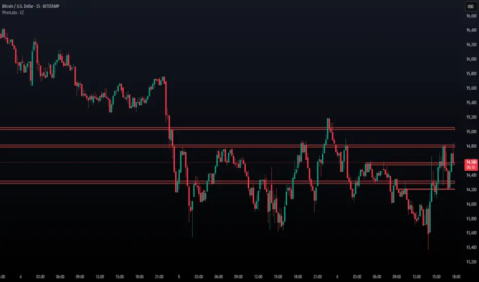
Approximate Entropy Zones [PhenLabs]Version: PineScript™ v6
Description
This indicator identifies periods of market complexity and randomness by calculating the Approximate Entropy (ApEn) of price action. As the movement of the market becomes complex, it means the current trend is losing steam and a reversal or consolidation is likely near. The indicator plots high-entropy periods as zones on your chart, providing a graphical suggestion to anticipate a potential market direction change. This indicator is designed to help traders identify favorable times to get in or out of a trade by highlighting when the market is in a state of disarray.
Points of Innovation
Advanced Complexity Analysis: Instead of relying on traditional momentum or trend indicators, this tool uses Approximate Entropy to quantify the unpredictability of price movements.
Dynamic Zone Creation: It automatically plots zones on the chart during periods of high entropy, providing a clear and intuitive visual guide.
Customizable Sensitivity: Users can fine-tune the ‘Entropy Threshold’ to adjust how frequently zones appear, allowing for calibration to different assets and timeframes.
Time-Based Zone Expiration: Zones can be set to expire after a specific time, keeping the chart clean and relevant.
Built-in Zone Size Filter: Excludes zones that form on excessively large candles, filtering out noise from extreme volatility events.
On-Chart Calibration Guide: A persistent note on the chart provides simple instructions for adjusting the entropy threshold, making it easy for users to optimize the indicator’s performance.
Core Components
Approximate Entropy (ApEn) Calculation: The core of the indicator, which measures the complexity or randomness of the price data.
Zone Plotting: Creates visual boxes on the chart when the calculated ApEn value exceeds a user-defined threshold.
Dynamic Zone Management: Manages the lifecycle of the zones, from creation to expiration, ensuring the chart remains uncluttered.
Customizable Settings: A comprehensive set of inputs that allow users to control the indicator’s sensitivity, appearance, and time-based behavior.
Key Features
Identifies Potential Reversals: The high-entropy zones can signal that a trend is nearing its end, giving traders an early warning.
Works on Any Timeframe: The indicator can be applied to any chart timeframe, from minutes to days.
Customizable Appearance: Users can change the color and transparency of the zones to match their chart’s theme.
Informative Labels: Each zone can display the calculated entropy value and the direction of the candle on which it formed.
Visualization
Entropy Zones: Shaded boxes that appear on the chart, highlighting candles with high complexity.
Zone Labels: Text within each zone that displays the ApEn value and a directional arrow (e.g., “0.525 ↑”).
Calibration Note: A small table in the top-right corner of the chart with instructions for adjusting the indicator’s sensitivity.
Usage Guidelines
Entropy Analysis
Source: The price data used for the ApEn calculation. (Default: close)
Lookback Length: The number of bars used in the ApEn calculation. (Default: 20, Range: 10-50)
Embedding Dimension (m): The length of patterns to be compared; a standard value for financial data. (Default: 2)
Tolerance Multiplier (r): Adjusts the tolerance for pattern matching; a larger value makes matching more lenient. (Default: 0.2)
Entropy Threshold: The ApEn value that must be exceeded to plot a zone. Increase this if too many zones appear; decrease it if too few appear. (Default: 0.525)
Time Settings
Analysis Timeframe: How long a zone remains on the chart after it forms. (Default: 1D)
Custom Period (Bars): The zone’s lifespan in bars if “Analysis Timeframe” is set to “Custom”. (Default: 1000)
Zone Settings
Zone Fill Color: The color of the entropy zones. (Default: #21f38a with 80% transparency)
Maximum Zone Size %: Filters out zones on candles that are larger than this percentage of their low price. (Default: 0.5)
Display Options
Show Entropy Label: Toggles the visibility of the text label inside each zone. (Default: true)
Label Text Position: The horizontal alignment of the text label. (Default: Right)
Show Calibration Note: Toggles the visibility of the calibration note in the corner of the chart. (Default: true)
Best Use Cases
Trend Reversal Trading: Identifying when a strong trend is likely to reverse or pause.
Breakout Confirmation: Using the absence of high entropy to confirm the strength of a breakout.
Ranging Market Identification: Periods of high entropy can indicate that a market is transitioning into a sideways or choppy phase.
Limitations
Not a Standalone Signal: This indicator should be used in conjunction with other forms of analysis to confirm trading signals.
Lagging Nature: Like all indicators based on historical data, ApEn is a lagging measure and does not predict future price movements with certainty.
Calibration Required: The effectiveness of the indicator is highly dependent on the “Entropy Threshold” setting, which needs to be adjusted for different assets and timeframes.
What Makes This Unique
Quantifies Complexity: It provides a numerical measure of market complexity, offering a different perspective than traditional indicators.
Clear Visual Cues: The zones make it easy to see when the market is in a state of high unpredictability.
User-Friendly Design: With features like the on-chart calibration note, the indicator is designed to be easy to use and optimize.
How It Works
Calculate Standard Deviation: The indicator first calculates the standard deviation of the source price data over a specified lookback period.
Calculate Phi: It then calculates a value called “phi” for two different pattern lengths (embedding dimensions ‘m’ and ‘m+1’). This involves comparing sequences of data points to see how many are “similar” within a certain tolerance (determined by the standard deviation and the ‘r’ multiplier).
Calculate ApEn: The Approximate Entropy is the difference between the two phi values. A higher ApEn value indicates greater irregularity and unpredictability in the data.
Plot Zones: If the calculated ApEn exceeds the user-defined ‘Entropy Threshold’, a zone is plotted on the chart.
Note: The “Entropy Threshold” is the most important setting to adjust. If you see too many zones, increase the threshold. If you see too few, decrease it.

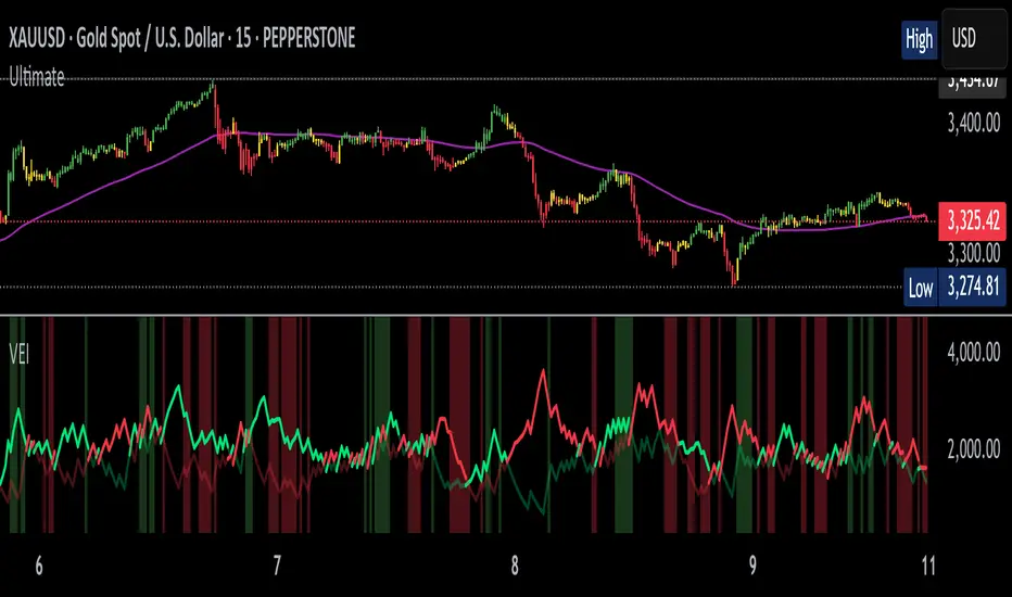
Volumetric Entropy IndexVolumetric Entropy Index (VEI)
A volume-based drift analyzer that captures directional pressure, trend agreement, and entropy structure using smoothed volume flows.
---
🧠 What It Does:
• Volume Drift EMAs : Shows buy/sell pressure momentum with adaptive smoothing.
• Dynamic Bands : Bollinger-style volatility wrappers react to expanding/contracting drift.
• Baseline Envelope : Clean structural white rails for mean-reversion zones or trend momentum.
• Background Shading : Highlights when both sides (up & down drift) are in agreement — green for bullish, red for bearish.
• Alerts Included : Drift alignment, crossover events, net drift shifts, and strength spikes.
---
🔍 What Makes It Different:
• Most volume indicators rely on bars, oscillators, or OBV-style accumulation — this doesn’t.
• It compares directional EMAs of raw volume to isolate real-time bias and acceleration.
• It visualizes the twisting tension between volume forces — not just price reaction.
• Designed to show when volatility is building inside the volume mechanics before price follows.
• Modular — every element is optional, so you can run it lean or fully loaded.
---
📊 How to Use It:
• Drift EMAs : Watch for one side consistently dominating — sharp spikes often precede breakouts.
• Bands : When they tighten and start expanding, it often signals directional momentum forming.
• Envelope Lines : Use as high-probability reversal or continuation zones. Bands crossing envelopes = potential thrust.
• Background Color : Green/red backgrounds confirm volume agreement. Can be used as a filter for other signals.
• Net Drift : Optional smoothed oscillator showing the difference between bullish and bearish volume pressure. Crosses above or below zero signal directional bias shifts.
• Drift Strength : Measures pressure buildup — spikes often correlate with large moves.
---
⚙️ Full Customization:
• Turn every layer on/off independently
• Modify all colors, transparencies, and line widths
• Adjust band width multiplier and envelope offset (%)
• Toggle bonus plots like drift strength and net baseline
---
🧪 Experimental Tools:
• Smoothed Net Drift trace
• Drift Strength signal
• Envelope lines and dynamic entropy bands with adjustable math
---
Built for signal refinement. Made to expose directional imbalance before the herd sees it.
Created by @Sherlock_Macgyver
Entropy Chart Analysis [PhenLabs]📊 Entropy Chart analysis -
Version: PineScript™ v6
📌 Description
The Entropy Chart indicator analysis applies Approximate Entropy (ApEn) to identify zones of potential support and resistance on your price chart. It is designed to locate changes in the market’s predictability, with a focus on zones near significant psychological price levels (e.g., multiples of 50). By quantifying entropy, the indicator aims to identify zones where price action might stabilize (potential support) or become randomized (potential resistance).
This tool automates the visualization of these key areas for traders, which may have the effect of revealing reversal levels or consolidation zones that would be hard to discern through traditional means. It also filters the signals by proximity to key levels in an attempt to reduce noise and highlight higher-probability setups. These dynamic zones adapt to changing market conditions by stretching, merging, and expiring based on user-inputted rules.
🚀 Points of Innovation
Combines Approximate Entropy (ApEn) calculation with price action near significant levels.
Filters zone signals based on proximity (in ticks) to predefined significant price levels (multiples of 50).
Dynamically merges overlapping or nearby zones to consolidate signals and reduce chart clutter.
Uses ApEn crossovers relative to its moving average as the core trigger mechanism.
Provides distinct visual coloring for bullish, bearish, and merged (mixed-signal) zones.
Offers comprehensive customization for entropy calculation, zone sensitivity, level filtering, and visual appearance.
🔧 Core Components
Approximate Entropy (ApEn) Calculation : Measures the regularity or randomness of price fluctuations over a specified window. Low ApEn suggests predictability, while high ApEn suggests randomness.
Zone Trigger Logic : Creates potential support zones when ApEn crosses below its average (indicating increasing predictability) and potential resistance zones when it crosses above (indicating increasing randomness).
Significant Level Filter : Validates zone triggers only if they occur within a user-defined tick distance from significant price levels (multiples of 50).
Dynamic Zone Management : Automatically creates, extends, merges nearby zones based on tick distance, and removes the oldest zones to maintain a maximum limit.
Zone Visualization : Draws and updates colored boxes on the chart to represent active support, resistance, or mixed zones.
🔥 Key Features
Entropy-Based S/R Detection : Uses ApEn to identify potential support (low entropy) and resistance (high entropy) areas.
Significant Level Filtering : Enhances signal quality by focusing on entropy changes near key psychological price points.
Automatic Zone Drawing & Merging : Visualizes zones dynamically, merging close signals for clearer interpretation.
Highly Customizable : Allows traders to adjust parameters for ApEn calculation, zone detection thresholds, level filter sensitivity, merging distance, and visual styles.
Integrated Alerts : Provides built-in alert conditions for the formation of new bullish or bearish zones near significant levels.
Clear Visual Output : Uses distinct, customizable colors for buy (support), sell (resistance), and mixed (merged) zones.
🎨 Visualization
Buy Zones : Represented by greenish boxes (default: #26a69a), indicating potential support areas formed during low entropy periods near significant levels.
Sell Zones : Represented by reddish boxes (default: #ef5350), indicating potential resistance areas formed during high entropy periods near significant levels.
Mixed Zones : Represented by bluish/purple boxes (default: #8894ff), formed when a buy zone and a sell zone merge, indicating areas of potential consolidation or conflict.
Dynamic Extension : Active zones are automatically extended to the right with each new bar.
📖 Usage Guidelines
Calculation Parameters
Window Length
Default: 15
Range: 10-100
Description: Lookback period for ApEn calculation. Shorter lengths are more responsive; longer lengths are smoother.
Embedding Dimension (m)
Default: 2
Range: 1-6
Description: Length of patterns compared in ApEn calculation. Higher values detect more complex patterns but require more data.
Tolerance (r)
Default: 0.5
Range: 0.1-1.0 (step 0.1)
Description: Sensitivity factor for pattern matching (as a multiple of standard deviation). Lower values require closer matches (more sensitive).
Zone Settings
Zone Lookback
Default: 5
Range: 5-50
Description: Lookback period for the moving average of ApEn used in threshold calculations.
Zone Threshold
Default: 0.5
Range: 0.5-3.0
Description: Multiplier for the ApEn average to set crossover trigger levels. Higher values require larger ApEn deviations to create zones.
Maximum Zones
Default: 5
Range: 1-10
Description: Maximum number of active zones displayed. The oldest zones are removed first when the limit is reached.
Zone Merge Distance (Ticks)
Default: 5
Range: 1-50
Description: Maximum distance in ticks for two separate zones to be merged into one.
Level Filter Settings
Tick Size
Default: 0.25
Description: The minimum price increment for the asset. Must be set correctly for the specific instrument to ensure accurate level filtering.
Max Ticks Distance from Levels
Default: 40
Description: Maximum allowed distance (in ticks) from a significant level (multiple of 50) for a zone trigger to be valid.
Visual Settings
Buy Zone Color : Default: color.new(#26a69a, 83). Sets the fill color for support zones.
Sell Zone Color : Default: color.new(#ef5350, 83). Sets the fill color for resistance zones.
Mixed Zone Color : Default: color.new(#8894ff, 83). Sets the fill color for merged zones.
Buy Border Color : Default: #26a69a. Sets the border color for support zones.
Sell Border Color : Default: #ef5350. Sets the border color for resistance zones.
Mixed Border Color : Default: color.new(#a288ff, 50). Sets the border color for mixed zones.
Border Width : Default: 1, Range: 1-3. Sets the thickness of zone borders.
✅ Best Use Cases
Identifying potential support/resistance near significant psychological price levels (e.g., $50, $100 increments).
Detecting potential market turning points or consolidation zones based on shifts in price predictability.
Filtering entries or exits by confirming signals occurring near significant levels identified by the indicator.
Adding context to other technical analysis approaches by highlighting entropy-derived zones.
⚠️ Limitations
Parameter Dependency : Indicator performance is sensitive to parameter settings ( Window Length , Tolerance , Zone Threshold , Max Ticks Distance ), which may need optimization for different assets and timeframes.
Volatility Sensitivity : High market volatility or erratic price action can affect ApEn calculations and potentially lead to less reliable zone signals.
Fixed Level Filter : The significant level filter is based on multiples of 50. While common, this may not capture all relevant levels for every asset or market condition. Accurate Tick Size input is essential.
Not Standalone : Should be used in conjunction with other analysis methods (price action, volume, other indicators) for confirmation, not as a sole basis for trading decisions.
💡 What Makes This Unique
Entropy + Level Context : Uniquely combines ApEn analysis with a specific filter for proximity to significant price levels (multiples of 50), adding locational context to entropy signals.
Intelligent Zone Merging : Automatically consolidates nearby buy/sell zones based on tick distance, simplifying visual analysis and highlighting stronger confluence areas.
Targeted Signal Generation : Focuses alerts and zone creation on specific market conditions (entropy shifts near key levels).
🔬 How It Works
Calculate Entropy : The script computes the Approximate Entropy (ApEn) of the closing prices over the defined Window Length to quantify price predictability.
Check Triggers : It monitors ApEn relative to its moving average. A crossunder below a calculated threshold (avg_apen / zone_threshold) indicates potential support; a crossover above (avg_apen * zone_threshold) indicates potential resistance.
Filter by Level : A potential zone trigger is confirmed only if the low (for support) or high (for resistance) of the trigger bar is within the Max Ticks Distance of a significant price level (multiple of 50).
Manage & Draw Zones : If a trigger is confirmed, a new zone box is created. The script checks for overlaps with existing zones within the Zone Merge Distance and merges them if necessary. Zones are extended forward, and the oldest are removed to respect the Maximum Zones limit. Active zones are drawn and updated on the chart.
💡 Note:
Crucially, set the Tick Size parameter correctly for your specific trading instrument in the “Level Filter Settings”. Incorrect Tick Size will make the significant level filter inaccurate.
Experiment with parameters, especially Window Length , Tolerance (r) , Zone Threshold , and Max Ticks Distance , to tailor the indicator’s sensitivity to your preferred asset and timeframe.
Always use this indicator as part of a comprehensive trading plan, incorporating risk management and seeking confirmation from other analysis techniques.
Entropy-Based Adaptive SuperTrendOverview:
Introducing the Entropy-Based Adaptive SuperTrend – a groundbreaking trading indicator designed to adapt dynamically to market conditions using market entropy. This enhanced SuperTrend indicator adjusts its sensitivity according to the level of chaos (or order) in price movements, providing more stable signals during volatile periods and more responsive signals when the market becomes orderly.
Key Features:
Entropy-Adaptive Mechanism: By incorporating an entropy measure, this indicator estimates the degree of unpredictability in the market. During high entropy periods (more chaotic), signals are made less sensitive, while during low entropy periods, the indicator reacts more quickly to price changes.
Adaptive ATR Multiplier: Unlike traditional SuperTrend indicators that use a fixed ATR multiplier, this version calculates a dynamic ATR multiplier based on the entropy score, ensuring more flexibility and adaptability in setting stop levels.
Visual Clarity: The indicator is overlayed on the price chart with customizable visual elements. The bullish and bearish trends are color-coded for ease of use, and optional entry signals ("L" for long and "S" for short) are plotted to clearly mark potential entry opportunities.
Alerts for Key Opportunities : Never miss an opportunity with built-in alerts for buy and sell signals. Traders can easily configure these alerts to be notified instantly when market conditions trigger a new trend.
How It Works:
Entropy Calculation: The entropy of the price data is calculated over a user-defined period, giving an indication of the degree of randomness in the price movements. The result is then smoothed to reduce noise and create a meaningful trend indication.
Dynamic ATR Adjustment: The ATR (Average True Range) multiplier, which controls the distance of the trailing stop, is adjusted based on the entropy score. This allows the SuperTrend line to widen in chaotic times, reducing false signals, while tightening in orderly times, allowing quicker trend captures.
Parameters Explained:
Entropy Settings: Control the sensitivity of entropy calculations, including the look-back period, number of bins for price distribution, and smoothing length.
Adaptive Settings: Adjust how the indicator adapts to different levels of entropy, including the adaptation period and the filtering weight.
SuperTrend Settings : Customize the ATR period and the dynamic multiplier range to fine-tune the trailing stops for your trading style.
Visual Settings: Choose your preferred colors for bullish and bearish trends, and decide if you want the entry labels displayed directly on the chart.
Use Cases:
Swing Traders can utilize the indicator to capture trend reversals while filtering out the noise during high entropy periods.
Intraday Traders can adapt the settings for shorter time frames to benefit from dynamic adjustments that reduce overtrading and false signals.
Risk Management: The entropy-based adaptive feature provides an edge in risk management by reducing sensitivity during times of increased chaos, thus helping to limit unnecessary trades.
How to Use It:
Look for entry labels ("L" for long, "S" for short) to identify potential opportunities.
Use the color-coded trendlines to determine market bias: greenish hue for bullish trends, reddish hue for bearish trends.
Customize the input settings to align with your preferred market timeframe and risk profile.
Alerts & Notifications:
Built-in alerts notify you of significant trend changes. Simply enable these alerts to receive updates when a new long or short opportunity is detected, helping you stay ahead without needing to watch the screen constantly.
Customization Tips:
Longer Timeframes : Increase the Entropy Period to better capture macro trends in high timeframe charts.
Higher Volatility Markets: Increase the ATR Max Multiplier to ensure stops are set farther away during high entropy.
Lower Volatility Markets: Use a lower ATR Base Multiplier and tighter entropy thresholds to capture rapid price movements.
Final Thoughts:
The Entropy-Based Adaptive SuperTrend indicator merges traditional trend-following logic with an adaptive mechanism driven by market entropy, aiming to address the challenges of whipsaws and false signals common in conventional SuperTrend setups. This indicator offers an intelligent and flexible way to track market trends, suitable for both beginners and experienced trade

Volume EntropyKey Components :
📍 Natural Logarithm Function : The script starts by employing a custom Taylor Series approximation for natural logarithms. This function serves to calculate entropy with higher accuracy than conventional methods, laying the foundation for further calculations.
📍 Entropy Calculation : The core of this indicator is its entropy function. It employs the custom natural log function to compute the randomness of the trading volume over a user-defined micro-pattern length, offering insights into market stability or volatility.
📍 Micro-Pattern Length : This is the parameter that sets the stage for the level of detail in the entropy calculation. Users can adjust it to suit different time frames or market conditions, thus customizing the indicator's sensitivity to randomness in trading volume.
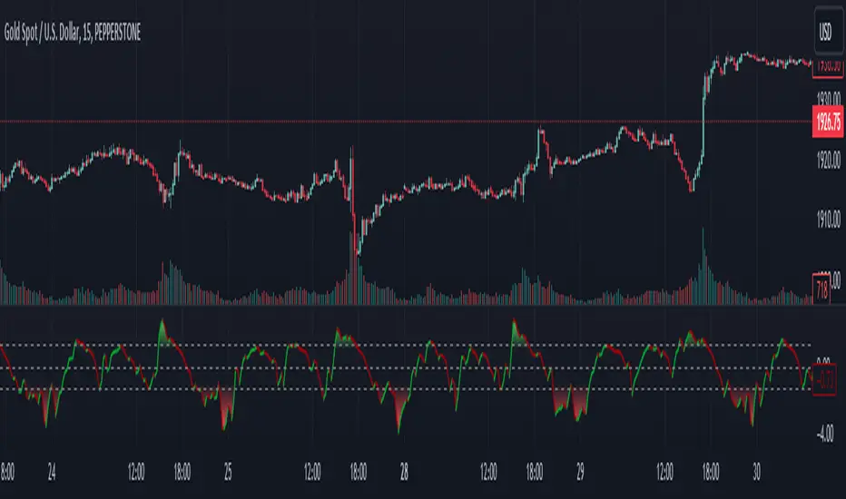
Entropy, Liquidity, and Momentum - ELMoELMo is a momentum trading strategy based on two concepts: entropy and liquidity
The core concept behind the strategy is twofold: trade based on reversals in momentum based on the strength of a trend, and trade when market liquidity is beneficial to the position.
Entries and exits are determined by first calculating Shannon entropy for the time series and applying various moving averages. Separately, the Hui-Heubel Liquidity Ratio (lhh) is calculated and applied as a filter. Finally, additional conditionals such as RSI are applied to reduce false entries.
Entropy is defined as the amount of 'randomness' in a system and in this application can be thought of as a measure of the strength or weakness of a trend. The main moving averages and visible components in ELMo represent the normalized entropy score of the 'close' value (0 is series minimum, 1 is maximum). lhh will measure illiquid/fragile markets with low values and liquid/resilient markets with a high value. In general, the strategy will prefer to enter long when liquidity is high and short when liquidity is low, based off of cross events in the displayed entropy moving averages. I have published lhh as a separate indicator but it is not required for this strategy to function.
Several settings can be configured inside the strategy, including long/short bias, lookback window, MA band lengths, RSI boundaries, and more, but I have tried to choose sensible defaults that work for a large variety of situations and equities. My preferred time scales are 1m 1h 4h 1d 1w 1mo but others may work fine. Trailing stops are implemented using configurable ATR values. Additional settings are available to limit entry times (default is set to US options market open/close), and backtesting start date.
The long strategy is generally more accurate than short. Since Pinescript does not have a way to manage long/short exposure in a hedged fashion, I prefer to run two separate instances of ELMo in long-only and short-only modes for signaling. I prefer to trade this strategy with a long bias using the short signals as indications of windows of weakness where hedging could be prudent.

Adaptive Two-Pole Super Smoother Entropy MACD [Loxx]Adaptive Two-Pole Super Smoother Entropy (Math) MACD is an Ehlers Two-Pole Super Smoother that is transformed into an MACD oscillator using entropy mathematics. Signals are generated using Discontinued Signal Lines.
What is Ehlers; Two-Pole Super Smoother?
From "Cycle Analytics for Traders Advanced Technical Trading Concepts" by John F. Ehlers
A SuperSmoother filter is used anytime a moving average of any type would otherwise be used, with the result that the SuperSmoother filter output would have substantially less lag for an equivalent amount of smoothing produced by the moving average. For example, a five-bar SMA has a cutoff period of approximately 10 bars and has two bars of lag. A SuperSmoother filter with a cutoff period of 10 bars has a lag a half bar larger than the two-pole modified Butterworth filter.Therefore, such a SuperSmoother filter has a maximum lag of approximately 1.5 bars and even less lag into the attenuation band of the filter. The differential in lag between moving average and SuperSmoother filter outputs becomes even larger when the cutoff periods are larger.
Market data contain noise, and removal of noise is the reason for using smoothing filters. In fact, market data contain several kinds of noise. I’ll group one kind of noise as systemic, caused by the random events of trades being exercised. A second kind of noise is aliasing noise, caused by the use of sampled data. Aliasing noise is the dominant term in the data for shorter cycle periods.
It is easy to think of market data as being a continuous waveform, but it is not. Using the closing price as representative for that bar constitutes one sample point. It doesn’t matter if you are using an average of the high and low instead of the close, you are still getting one sample per bar. Since sampled data is being used, there are some dSP aspects that must be considered. For example, the shortest analysis period that is possible (without aliasing)2 is a two-bar cycle.This is called the Nyquist frequency, 0.5 cycles per sample.A perfect two-bar sine wave cycle sampled at the peaks becomes a square wave due to sampling. However, sampling at the cycle peaks can- not be guaranteed, and the interference between the sampling frequency and the data frequency creates the aliasing noise.The noise is reduced as the data period is longer. For example, a four-bar cycle means there are four samples per cycle. Because there are more samples, the sampled data are a better replica of the sine wave component. The replica is better yet for an eight-bar data component.The improved fidelity of the sampled data means the aliasing noise is reduced at longer and longer cycle periods.The rate of reduction is 6 dB per octave. My experience is that the systemic noise rarely is more than 10 dB below the level of cyclic information, so that we create two conditions for effective smoothing of aliasing noise:
1. It is difficult to use cycle periods shorter that two octaves below the Nyquist frequency.That is, an eight-bar cycle component has a quantization noise level 12 dB below the noise level at the Nyquist frequency. longer cycle components therefore have a systemic noise level that exceeds the aliasing noise level.
2. A smoothing filter should have sufficient selectivity to reduce aliasing noise below the systemic noise level. Since aliasing noise increases at the rate of 6 dB per octave above a selected filter cutoff frequency and since the SuperSmoother attenuation rate is 12 dB per octave, the Super- Smoother filter is an effective tool to virtually eliminate aliasing noise in the output signal.
What are DSL Discontinued Signal Line?
A lot of indicators are using signal lines in order to determine the trend (or some desired state of the indicator) easier. The idea of the signal line is easy : comparing the value to it's smoothed (slightly lagging) state, the idea of current momentum/state is made.
Discontinued signal line is inheriting that simple signal line idea and it is extending it : instead of having one signal line, more lines depending on the current value of the indicator.
"Signal" line is calculated the following way :
When a certain level is crossed into the desired direction, the EMA of that value is calculated for the desired signal line
When that level is crossed into the opposite direction, the previous "signal" line value is simply "inherited" and it becomes a kind of a level
This way it becomes a combination of signal lines and levels that are trying to combine both the good from both methods.
In simple terms, DSL uses the concept of a signal line and betters it by inheriting the previous signal line's value & makes it a level.
Included:
Bar coloring
Alerts
Signals
Loxx's Expanded Source Types

Basic Shannon Entropy & DerivativesThis script performs the basic Shannon entropy on the closing value of the stock. Additionally, it performs the trailing first and second derivatives of the Shannon Entropy, giving you more information about its movement.
You can change the "Source" to be whatever value you like.

ProbabilityLibrary "Probability"
erf(value) Complementary error function
Parameters:
value : float, value to test.
Returns: float
ierf_mcgiles(value) Computes the inverse error function using the Mc Giles method, sacrifices accuracy for speed.
Parameters:
value : float, -1.0 >= _value >= 1.0 range, value to test.
Returns: float
ierf_double(value) computes the inverse error function using the Newton method with double refinement.
Parameters:
value : float, -1. > _value > 1. range, _value to test.
Returns: float
ierf(value) computes the inverse error function using the Newton method.
Parameters:
value : float, -1. > _value > 1. range, _value to test.
Returns: float
complement(probability) probability that the event will not occur.
Parameters:
probability : float, 0 >=_p >= 1, probability of event.
Returns: float
entropy_gini_impurity_single(probability) Gini Inbalance or Gini index for a given probability.
Parameters:
probability : float, 0>=x>=1, probability of event.
Returns: float
entropy_gini_impurity(events) Gini Inbalance or Gini index for a series of events.
Parameters:
events : float , 0>=x>=1, array with event probability's.
Returns: float
entropy_shannon_single(probability) Entropy information value of the probability of a single event.
Parameters:
probability : float, 0>=x>=1, probability value.
Returns: float, value as bits of information.
entropy_shannon(events) Entropy information value of a distribution of events.
Parameters:
events : float , 0>=x>=1, array with probability's.
Returns: float
inequality_chebyshev(n_stdeviations) Calculates Chebyshev Inequality.
Parameters:
n_stdeviations : float, positive over or equal to 1.0
Returns: float
inequality_chebyshev_distribution(mean, std) Calculates Chebyshev Inequality.
Parameters:
mean : float, mean of a distribution
std : float, standard deviation of a distribution
Returns: float
inequality_chebyshev_sample(data_sample) Calculates Chebyshev Inequality for a array of values.
Parameters:
data_sample : float , array of numbers.
Returns: float
intersection_of_independent_events(events) Probability that all arguments will happen when neither outcome
is affected by the other (accepts 1 or more arguments)
Parameters:
events : float , 0 >= _p >= 1, list of event probabilities.
Returns: float
union_of_independent_events(events) Probability that either one of the arguments will happen when neither outcome
is affected by the other (accepts 1 or more arguments)
Parameters:
events : float , 0 >= _p >= 1, list of event probabilities.
Returns: float
mass_function(sample, n_bins) Probabilities for each bin in the range of sample.
Parameters:
sample : float , samples to pool probabilities.
n_bins : int, number of bins to split the range
@return float
cumulative_distribution_function(mean, stdev, value) Use the CDF to determine the probability that a random observation
that is taken from the population will be less than or equal to a certain value.
Or returns the area of probability for a known value in a normal distribution.
Parameters:
mean : float, samples to pool probabilities.
stdev : float, number of bins to split the range
value : float, limit at which to stop.
Returns: float
transition_matrix(distribution) Transition matrix for the suplied distribution.
Parameters:
distribution : float , array with probability distribution. ex:.
Returns: float
diffusion_matrix(transition_matrix, dimension, target_step) Probability of reaching target_state at target_step after starting from start_state
Parameters:
transition_matrix : float , "pseudo2d" probability transition matrix.
dimension : int, size of the matrix dimension.
target_step : number of steps to find probability.
Returns: float
state_at_time(transition_matrix, dimension, start_state, target_state, target_step) Probability of reaching target_state at target_step after starting from start_state
Parameters:
transition_matrix : float , "pseudo2d" probability transition matrix.
dimension : int, size of the matrix dimension.
start_state : state at which to start.
target_state : state to find probability.
target_step : number of steps to find probability.

Alpha Trading - Absolute Mean Entropy with A2 EPPAbsolute Mean Entropy with Alpha Squared Entropy Price Percentile
Entropy
The history of the word ―entropy can be traced back to 1865 when the German physicist Rudolf Clausius tried to give a new name to irreversible heat loss, what he previously called ―equivalent-value.
The word ―entropy was chosen because in Greek, “en+tropein” means “content transformative” or “transformation content”
Since then, entropy has played an important role in thermodynamics and many other scientific fields. Being defined as the sum of “heat supplied” divided by “temperature” it is central to the Second Law of Thermodynamics. It also helps measure the amount of order and disorder and/or chaos.
The application of entropy in finance can be regarded as an extension of “Information Entropy” and “Probability Entropy”
Entropy in Finance can be used in many ways such as Asset Selection, Asset Diversification, Measure an Assets Risk, inputs into Options pricing. While Entropy started in the field of Thermodynamics as aforementioned it has also found a home in Finance. However, studies with entropy in the field of Finance are still in their infancy.
• Entropy is a measure of randomness. Entropy is used to help model and represent the degree of uncertainty of a random variable.
• Entropy is used by financial analysts and market technicians to determine the chances of a specific type of behavior by a security or market.
• Entropy has long been a source of study and debate by market analysts and traders. It is used in quantitative analysis and can help predict the probability that a security will move in a certain direction or according to a certain pattern.
The concept of Entropy is explored in the book "A Random Walk Down Wall Street."
Entropy is plotted below the axis with negative values. Entropy can also colorize the candle color if selected.
R-squared (The Coefficient of Determination)
R-squared is a statistical measurement that examines how differences in one variable can be explained by the difference in a second variable, when predicting the outcome of a given event.
In other words, this coefficient, which is more commonly known as R-squared (or R2), assesses how strong the linear relationship is between two variables, and is heavily relied on by researchers when conducting trend analysis.
To cite an example of its application, this coefficient may contemplate the following question: if an indicator becomes pregnant on a certain day, what is the likelihood that this indicator would deliver a new indicator on a particular date in the future? In this scenario, this metric aims to calculate the correlation between two related events: conception of the indicator and the birth of the indicator.
• The coefficient of determination is a complex idea centered on the statistical analysis of models for data.
• The coefficient of determination is used to explain how much variability of one factor can be caused by its relationship to another factor.
• This coefficient is commonly known as R-squared (or R2) and is sometimes referred to as the "goodness of fit."
• This measure is represented as a value between 0.0 and 1.0, where a value of 1.0 indicates a perfect fit, and is thus a highly reliable model for future forecasts, while a value of 0.0 would indicate that the model fails to accurately model the data at all.
R2 and Price
The hypothesis that R2 is related to investors’ biases in processing information.
This theory motivates an empirical hypothesis that stocks with lower R2 should exhibit more pronounced overreaction-driven price momentum.
Alpha Trading AME/A2 EPP Settings
Settings for AME (Absolute Mean Entropy)
Length: Sample size.
Use as Barcolor: AME color as Price Action Candle color.
Show Entropy Flashes: If absolute value of entropy is very low, it gives yellow color for AME and Price Action Candle color if selected.
Band StdDev: (2 times) AME StdDev bands.1st and 2nd default.
Exponential Weighted Entropy: Weights the AME exponentially, is more reactive, but more noise.
Settings for EPP (Entropy Price Percentile)
Percentile Period: lookback for percentile range(relevant for flashes)
Background flashes: if EPP is below threshold default is below 10%, Flashes green in the background.
Std.err bands period: default 3 and multiplier 1.
EPP Column Meanings
Bright Green: Returns above the mean and increasing.
Dark Green: Returns above the mean and decreasing.
Bright Red: Returns below the mean and increasing.
Dark Red: Returns below the mean and decreasing.
Basic Trade Signal
Long – Value of AME is low, as you see EPP increasing with a coloration of green consider taking a long if you have confluence with other Alpha Trading Indicators.
Short – Value of AME is low, as you see EPP increasing with a coloration of red consider taking a short if you have confluence with other Alpha Trading Indicators.
The Chart below is showing Entries, Exponential Weighting input turned on, Percentile Period set to 30 instead of default 100, everything else is Default....
When using other Alpha Trading indicators in confluence, there are other entries available when the indicator isn't flashing and the indicator still supports the move.
References
www.investopedia.com
www.investopedia.com
www.wallstreetmojo.com
byjus.com
www.investopedia.com
en.wikipedia.org
papers.ssrn.com

Function - Entropy Gini Indexfunction to retrieve Gini Impurity / Gini Index.
reference:
- victorzhou.com
- en.wikipedia.org

Function - Shannon Entropyfunctions for shannon's entropy
reference:
- en.wiktionary.org
- machinelearningmastery.com

[Max] Volume Entropy Divergence FilteredAn indicator that represent in 3 line my Volume Entropy Divergence Heatmap indicator.
I've use a very basic sum with some weights like this : Long therm > Mid therm > short Therm, But short and mid therm can still have influence.
Some people did request this indicator to be able to use the heatmap in there indicators with the new tradingview link function. There still a problem that will be the subject of a future update, when the divergence is to high it's often mean that instead of a divergence, we have a continuation or a parabolic.
This indicator still also need a location checker to try to don't short the bottom.
There is 3 lines, 2 are the sum of the negative/positive divergences.
The third one is the result off a karman volatility filter, with differents weigths for each line off the heatmap, it can easily used to find reversals.
You have some options to play with the volatility filter, the defaults settings are the ones I think is the best.
This script will still private for the same reasons raised in the original heatmap.
My policy : If you can provide me nice updates, I will give you the source code, if within 3 month I don't use it anymore it will pass in public.
If you have any improvement idears I will be please to ear them.
Have a nice day !
Max

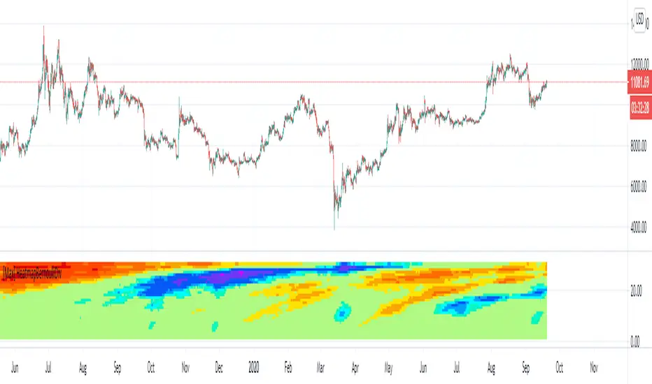
[Max] Volume Entropy Divergence HeatmapA divergence between volume and price indicator, based on custom filter function.
Each lines represent a length on wich the divergence is calculated. It goes to 60 len a the base to 2000 at the high. ( You have to decrease the timeframe if your looking on a new chart).
Colors represent a level of the oscillator who is calculated for each lengths.
What can you find, reversals, confirmation of continuation, divergences between volume and price,.. (if you find other usages I will be happy to hear it and share the code).
I recommand to be attentive to lower timeframes and confirm with higher ones and be attentive between different kind of clouds there is.
You are in charge to figure out how to use it, if you have some doubts on something you can DM me but I will not teach my way to use it.
It provide for me nice transformations, nice enough to share this indicator in private.
Big thanks to @midtownsk8rguy for the heatmap color function.
Have a nice daytrading all !

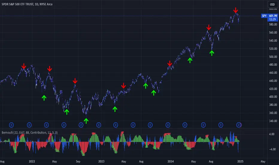
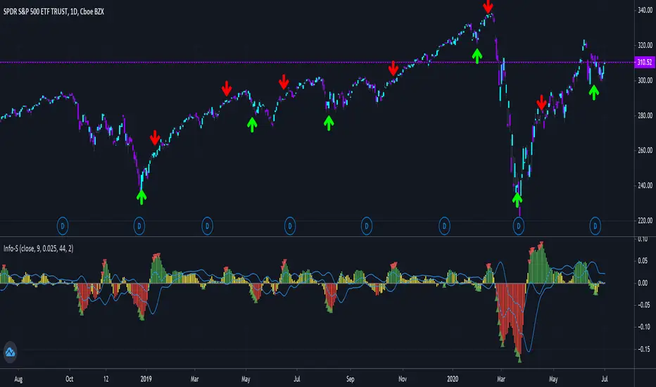
Bernoulli Process - Binary Entropy FunctionThis indicator is the Bernoulli Process or Wikipedia - Binary Entropy Function . Within Information Theory, Entropy is the measure of available information, here we use a binary variable 0 or 1 (P) and (1-P) (Bernoulli Function/Distribution), and combined with the Shannon Entropy measurement. As you can see below, it produces some wonderful charts and signals, using price, volume, or both summed together. The chart below shows you a couple of options and some critical details on the indicator. The best part about this is the simplicity, all of this information in a couple of lines of code.
Using the indicator:
The longer the Entropy measurement the more information you are capturing, so the analogy is, the shorter the signal, the less information you have available to utilize. You'll run into your Nyquist frequencies below a length of 5. I've found values between 9 and 22 work well to gather enough measurements. You also have an averaging summation that measures the weight or importance of the information over the summation period. This is also used for highlighting when you have an information signal above the 5% level (2 sigma) and then can be adjusted using the Percent Rank Variable. Finally, you can plot the individual signals (Price or Volume) to get another set of measurements to utilize. As can be seen in the chart below, the volume moves before price (but hopefully you already knew that)
At its core, this is taking the Binary Entropy measurement (using a Bernoulli distribution) for price and volume. I've subtracted the volume from the price so that you can use it like a MACD, also for shorter time frames (7, 9, 11) you can get divergences on the histogram. These divergences are primarily due to the weekly nature of the markets (5 days, 10 days is two weeks,...so 9 is measuring the last day of the past two weeks...so 11 is measuring the current day and the past two weeks).
Here are a couple of other examples, assuming you just love BTC, Stocks, or FOREX. I fashioned up a strategy to show the potential of the indicator.
BTC-Strategy
Stock-Strategy (#loveyouNFLX)
FOREX - (for everyone hopped up on 40X leverage)
Shannon Entropy V2Version 2, Shannon Entropy
This update includes both a deadband (Plotting Optional) and PercentRank Indicating.
Here is a unique way of looking at your price & volume information. Utilize the calculated value of "Shannon Entropy". This is a measure of "surprise" in the data, the larger the move or deviation from the most probable value, the higher the new information gain. What I think is so interesting about this value, is the smoothness that it displays the information without using moving averages. There is a lot of meat on this bone to be incorporated in other scripts.
H = -sum(prob(i) * log_base2(prob(i)))
I've included the typical way that I've been experimenting with this, which is the difference between the volume information and price information. I've included the option to turn either price or volume data off to see the Shannon Entropy value of either value. There are a ton of complex scripts out there trying to do what this calculation is doing in 3 lines. As with anything, there are no free lunches, so you can nicely see as you lower the lengths you'll quickly learn where your nyquist frequencies are at, you'll want to work at about double the noisy value at a minimum.
Using this script is based on "Information" and it highlights places that need your attention, either because there is a large amount of change (new information) or there is minimal new information (complacency, institutional movements). Buy and Sell points are up to the user, this is just showing you where you need to provide some attention.
You can use it with or without volume data, you can also isolate either the source and volume. Below are some options for printing:
It can also with BTC (better with volume data)
Big shoutout to yatrader2 for great Shannon Entropy discussions.
And to Picte/ for his interesting inspiration STOCH-HVP-picte
Shannon EntropyHere is a unique way of looking at your price & volume information. Utilize the calculated value of "Shannon Entropy". This is a measure of "surprise" in the data, the larger the move or deviation from the most probable value, the higher the new information gain. What I think is so interesting about this value, is the smoothness that it displays the information without using moving averages. There is a lot of meat on this bone to be incorporated in other scripts.
H = -sum(prob(i) * log_base2(prob(i)))
I've included the typical way that I've been experimenting with this, which is the difference between the volume information and price information. I've included the option to turn either price or volume data off to see the Shannon Entropy value of either value. There are a ton of complex scripts out there trying to do what this calculation is doing in 3 lines.
As with anything, there are no free lunches, so you can nicely see as you lower the lengths you'll quickly learn where your nyquist frequencies are at, you'll want to work at about double the noisy value at a minimum.

P-Signal v2.0Description.
-------------
P-Signal v.2.0 is a modified and improved version of an earlier published P-Signal. This version allows to observe
the signal image for a multi frame - a specific set of periods. In this version it is {T, 2T, 4T, 8T, 16T},
where T equals the “working” time i.e. period for which a chart is observed. For example, if T=5m, one can observe
P-Signal not only for 5m period (ocher curve) but also an average image of P-Signal for 5m, 10m, 20m, 40m, 80m
periods (grey curve) without switching over frames.
Moreover p-Signal v2.0 allows to catch "winning" combinations with help of alerts. When alert is active, you'll receive
a notification if combination exists after working frame was closed. There are two combinations in this version:
“High” and “Straight”. The terminology is borrowed from poker game to more easily present trading ideas.
For example: " EUR.USD Straight SHORT on 4h " and so on.
The “High” alert corresponds to absolute value of Gauss error function of working frame (T) not less the value which
is defined by Alert on “High” parameter. The “Straight” combination is registered if same sign signals (poker “flush”)
are observed simultaneously over set of periods. The rank of “Straight” combination is defined by T and Alert on “Straight”
parameter. This combination is less frequent, but stronger the previous one if parameters are chosen reasonably.
Value of parameters depend on T. The lower T the closer parameters to 1. By default “High” equals to 0.98 and
“Straight” equals to 0.85. Both for T=1m. The other parameters correspond to the first version.
Important ! For correct operation T should not exceed the values of hourly time frames!
Good luck!
