NAIFCHART_Fresh Algo v24# NAIFCHART Fresh Algo v24: Advanced Multi-Mode Trading System Analysis
I recently discovered this sophisticated trading system through the active community at t.me and wanted to share a detailed analysis of the NAIFCHART Fresh Algo v24 indicator. This represents an advanced evolution of multi-component trading systems that adapts to various market conditions through sophisticated operational configurations and enhanced analytical capabilities.
## Primary Signal Generation Framework
The Fresh Algo v24 operates through two fundamental signal generation approaches that accommodate different market perspectives and trading philosophies. The Trending Signals Mode serves as the primary trend-following mechanism, combining Wave Trend Oscillator analysis with Supertrend directional signals and Squeeze Momentum breakout detection. This mode incorporates ADX filtering that requires values exceeding 20 to ensure sufficient trend strength exists before signal activation, making it particularly effective during sustained directional market movements where momentum persistence creates profitable trading opportunities.
The Contrarian Signals Mode provides an alternative approach targeting reversal opportunities through extreme market condition identification. This mode activates when the Wave Trend Oscillator reaches critical threshold levels, specifically when readings surpass 65 indicating potential bearish reversal conditions or drop below 35 suggesting bullish reversal opportunities. This methodology proves valuable during overextended market phases where mean reversion becomes statistically probable.
## Advanced Filtering Mechanisms
The system incorporates multiple sophisticated filtering mechanisms designed to enhance signal quality and reduce false positive occurrences. The High Volume Filter requires volume expansion confirmation before signal activation, utilizing exponential moving average calculations to ensure institutional participation accompanies price movements. This filter substantially improves signal reliability by eliminating low-conviction breakouts that lack adequate volume support from professional market participants.
The Strong Filter provides additional trend confirmation through 200-period exponential moving average analysis. Long position signals require price action above this benchmark level, while short position signals necessitate price action below it. This ensures strategic alignment with longer-term trend direction and reduces the probability of trading against major market movements that could invalidate shorter-term signals.
## Cloud Filter Configuration System
The Fresh Algo v24 offers four distinct cloud filter configurations, each optimized for specific trading timeframes and market approaches. The Smooth Cloud Filter utilizes the mathematical relationship between 150-period and 250-period exponential moving averages, providing stable trend identification suitable for position trading strategies. This configuration generates signals exclusively when price action aligns with cloud direction, creating a more deliberate but highly reliable signal generation process.
The Swing Cloud Filter employs modified Supertrend calculations with parameters specifically optimized for swing trading timeframes. This filter achieves optimal balance between responsiveness and stability, adapting effectively to medium-term price movements while filtering excessive market noise that typically affects shorter-term analytical systems.
For active intraday traders, the Scalping Cloud Filter utilizes accelerated Supertrend calculations designed to capture rapid trend changes effectively. This configuration provides enhanced signal generation frequency suitable for compressed timeframe strategies. The advanced Scalping+ Cloud Filter incorporates Hull Moving Average confirmation, delivering maximum responsiveness for ultra-short-term trading while maintaining signal quality through additional momentum validation processes.
## Specialized Assistant Functionality
The system includes two distinct assistant modes that provide supplementary market analysis capabilities. The Trend Assistant Mode activates advanced cloud analysis overlays that display dynamic support and resistance zones calculated through adaptive volatility algorithms. These levels automatically adjust to current market conditions, providing visual guidance for identifying trend continuation patterns and potential reversal areas with mathematical precision.
The Trend Tracker Mode concentrates on long-term trend identification by displaying major exponential moving averages with color-coded fill areas that clarify directional bias. This mode maintains visual simplicity while providing comprehensive trend context evaluation, enabling traders to quickly assess broader market direction and align shorter-term strategies accordingly.
## Dynamic Risk Management System
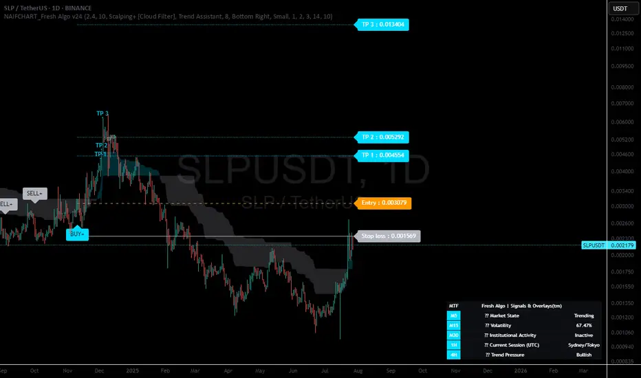
The integrated risk management system automatically adapts across all operational modes, calculating stop loss and take profit targets using Average True Range multiples that adjust to current market volatility. This approach ensures consistent risk parameters regardless of selected operational mode while maintaining relevance to prevailing market conditions.
Stop loss placement occurs at 3x ATR distance from entry points, while three progressive take profit targets establish at 1x, 2x, and 3x ATR multiples respectively. The system automatically updates these levels upon trend direction changes, ensuring current market volatility influences all risk calculations and maintains appropriate risk-reward ratios throughout trade management.
## Comprehensive Market Analysis Dashboard
The sophisticated dashboard provides real-time market analysis including volatility measurements, institutional activity assessment, and multi-timeframe trend evaluation across five-minute through four-hour periods. This comprehensive market context assists traders in selecting appropriate operational modes based on current market characteristics rather than relying exclusively on historical performance data.
The multi-timeframe analysis ensures mode selection considers broader market context beyond the primary trading timeframe, improving overall strategic alignment and reducing conflicts between different temporal market perspectives. The dashboard displays market state classification, volatility percentages, institutional activity levels, current trading session information, and trend pressure indicators.
## Enhanced Trading Assistants
The Fresh Algo v24 includes specialized trading assistant features that complement the primary signal generation system. The Reversal Dot functionality identifies potential reversal points through Wave Trend Oscillator analysis, displaying small circles when crossover conditions occur at extreme levels. These reversal indicators provide early warning signals for potential trend changes before they appear in the primary signal system.
The Dynamic Take Profit Labels feature automatically identifies optimal profit-taking opportunities through RSI threshold analysis, marking potential exit points at 70, 75, and 80 levels for long positions and 30, 25, and 20 levels for short positions. This automated profit management system helps traders optimize exit timing without requiring constant manual monitoring.
## Advanced Alert System
The comprehensive alert system accommodates all operational modes while providing granular notification control for various signal types and risk management events. Traders can configure separate alerts for normal buy signals, strong buy signals, normal sell signals, strong sell signals, stop loss triggers, and individual take profit target achievements.
Cloud crossover alerts notify traders when trend direction changes occur, providing early indication of potential strategy adjustments. The alert system includes detailed trade setup information, timeframe data, and relevant entry and exit levels, ensuring traders receive complete context for informed decision-making.
## Technical Foundation Architecture
The Fresh Algo v24 combines multiple proven technical analysis components including Wave Trend Oscillator for momentum assessment, Supertrend for directional bias determination, Squeeze Momentum for volatility analysis, and various exponential moving averages for trend confirmation. Each component contributes specific market insights while the unified system provides comprehensive market evaluation through their mathematical integration.
The multi-component approach reduces dependency on individual indicator limitations while leveraging the analytical strengths of each technical tool. This creates a robust analytical framework capable of adapting to diverse market conditions through appropriate mode selection and parameter optimization.
## Implementation Strategy Considerations
Successful implementation requires careful matching of operational modes to prevailing market conditions and individual trading objectives. Trending modes demonstrate optimal performance during directional markets with sustained momentum characteristics, while contrarian modes excel during range-bound or overextended market conditions where reversal probability increases.
The cloud filter configurations provide varying degrees of confirmation strength, with smoother settings reducing false signal occurrence at the expense of some responsiveness to price changes. Traders must balance signal quality against signal frequency based on their risk tolerance and available trading time.
## Community Development Framework
This indicator represents ongoing community-driven development through the team at t.me where continuous discussions focus on optimization techniques, practical implementation strategies, and real-world performance feedback. The collaborative development approach ensures the system remains relevant to actual market conditions while incorporating insights from active professional traders.
Understanding these operational modes and their specific applications enables traders to optimize the NAIFCHART Fresh Algo v24 system according to their particular requirements while maintaining consistent risk management principles across all market environments. The inherent flexibility in the multi-mode design allows strategic adaptation to changing market conditions without requiring complete methodology overhaul.
---
*Source: NAIFCHART Fresh Algo v24 available through t.me
Indicators and strategies
Enhanced Predator Suite🎯 Simple Predator Suite Guide - What You See on Your Chart
📍 What to Look For RIGHT NOW on Your BTC Chart
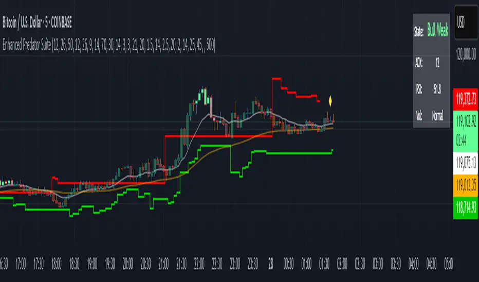
1. BAR COLORS (Most Important)
Look at the color of each price bar:
🟢 BRIGHT GREEN = BUY SIGNAL (Bull Strong)
🟢 LIGHT GREEN = Weak buy (be careful)
🟠 ORANGE = Weak sell (take profits)
🔴 RED = SELL SIGNAL (Bear Strong)
⚫ GRAY = DON'T TRADE (choppy market)
2. TRIANGLE SIGNALS
These are your entry points:
▲ GREEN TRIANGLE UP = Enter LONG (buy) on next bar
▼ RED TRIANGLE DOWN = Enter SHORT (sell) on next bar
3. TRAILING STOP LINES
🟢 GREEN LINE = Exit your long trades if price hits this
🔴 RED LINE = Exit your short trades if price hits this
🚀 SUPER SIMPLE TRADING METHOD
FOR LONG TRADES (BUYING)
Wait for a green triangle ▲ to appear
Buy on the next candle
Set stop loss below the green line
Take profit when bars turn orange or red
FOR SHORT TRADES (SELLING)
Wait for a red triangle ▼ to appear
Sell on the next candle
Set stop loss above the red line
Take profit when bars turn light green or bright green
WHEN TO STAY OUT
Gray bars = Market is confused, don't trade
No triangles = No clear entry signal
Price far from lines = You missed the move
🚫 COMMON MISTAKES TO AVOID
DON'T Do These Things:
❌ Trade during gray bars (choppy market)
❌ Enter without seeing a triangle signal
❌ Ignore the trailing stop lines
❌ Trade with big position sizes at first
❌ Chase price if you missed the triangle
DO These Instead:
✅ Wait patiently for clear triangle signals
✅ Always use the stop loss lines
✅ Start with tiny position sizes
✅ Take profits when bar colors change
✅ Stay out during gray bar periods
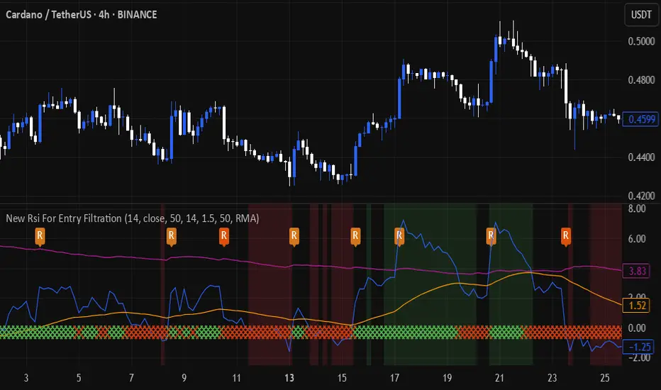
New Rsi For Entry FiltrationThis indicator, which is based on the RSI indicator, is written to prevent you from entering the wrong trade. Its operation is very simple. Enter a long trade when both the main area and the lower ribbon are green. Also, for a short trade, both the main area and the lower ribbon are red. The purple line also shows the stop loss level based on ATR. It is not advisable to enter the trade at the points indicated by R because the candlestick length is long.
NAIFCHART_Osc+ ST+sqzmom# NAIFCHART Multi-Component Indicator: Trading Analysis Guide
## Overview
The NAIFCHART Osc+ ST+sqzmom indicator combines three proven technical analysis tools into a unified trading system. This indicator was developed and shared by the trading community at t.me providing traders with comprehensive market analysis through integrated momentum, trend, and volatility assessment.
## Core Components
**Wave Trend Oscillator**: Identifies overbought and oversold conditions using exponential moving averages. Key levels include overbought zones at 60 and 53, with oversold areas at -60 and -53. Crossover signals between the two oscillator lines generate entry opportunities, displayed as colored circles on the chart.
**Supertrend Indicator**: Determines market direction using Average True Range calculations with a 2.5 factor and 10-period ATR. Green lines indicate uptrends while red lines signal downtrends. The indicator adapts to market volatility, providing reliable trend identification across different market conditions.
**Squeeze Momentum**: Compares Bollinger Bands with Keltner Channels to identify consolidation periods and breakouts. Black squares indicate squeeze conditions (low volatility), green triangles signal upward breakouts, and red triangles mark downward breakouts.
## Trading Signals
**Long Entry Signals**: Green triangles from Squeeze Momentum, Supertrend line turning green, and bullish crossovers in Wave Trend Oscillator from oversold levels.
**Short Entry Signals**: Red triangles from Squeeze Momentum, Supertrend line turning red, and bearish crossovers in Wave Trend Oscillator from overbought levels.
## Risk Management Features
The indicator automatically calculates risk management levels using ATR-based calculations. Stop losses are positioned at 3x ATR distance, while three progressive take profit targets are set at 1x, 2x, and 3x ATR multiples. All levels are clearly displayed on the chart with colored lines and labels.
When trend direction changes, previous levels are automatically cleared and new calculations are generated, ensuring current market conditions are reflected in all risk parameters.
## Alert System
Comprehensive alerts include trend changes with complete trade setup details, squeeze release notifications for breakout opportunities, and trend weakness warnings for position management. Alert messages contain trading pair information, timeframe data, and all relevant entry and exit levels.
## Implementation Guidelines
**Timeframe Selection**: Higher timeframes (4-hour, daily) provide reliable signals for position trading. One-hour charts work well for day trading, while 15-30 minute timeframes enable scalping with enhanced risk management requirements.
**Risk Management**: Limit risk to 1-2% of capital per trade using the calculated stop loss levels for position sizing. Implement partial profit-taking at each target level while adjusting stops to protect gains.
**Market Adaptation**: The indicator's ATR-based calculations automatically adjust to market volatility. During high volatility periods, levels widen appropriately, while low volatility conditions result in tighter risk management parameters.
## Best Practices
Combine indicator signals with key support and resistance analysis for enhanced validation. Monitor volume to confirm breakout strength, particularly when Squeeze Momentum signals develop. Maintain awareness of economic events that may influence market behavior independent of technical signals.
The multi-component design provides internal confirmation through multiple signal alignment requirements, reducing false signals while maintaining reasonable trade frequency for active strategies.
## Community Resources
Access ongoing education and strategy discussions through the source community at t.me where traders share market analysis and optimization techniques for this indicator system.
## Conclusion
The NAIFCHART indicator offers a systematic approach to market analysis through proven technical components. Success requires understanding each element's functionality and implementing proper risk management principles. The community-driven development ensures practical relevance and ongoing support for traders seeking comprehensive market analysis tools.
Practice with demo accounts before live implementation to develop familiarity with signal interpretation and trade management procedures. The indicator's systematic approach reduces emotional decision-making while providing clear guidelines for entry, management, and exit strategies across various market conditions.

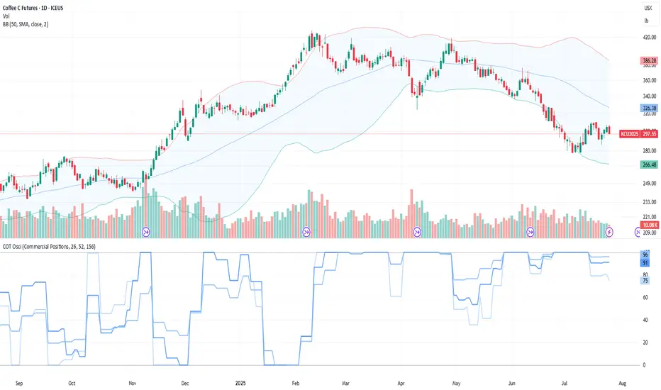
COT Comm OsciDescription
The COT Comm Osci is a sentiment oscillator based on net positions from the weekly Commitments of Traders (COT) report.
It transforms net positions of Commercials, Noncommercials, or Nonreportables into a 0–100 index.
A value of 100 = highest net position within the selected timeframe.
A value of 0 = lowest net position.
You can define three historical intervals (e.g. 26/ 52 / 156 weeks).
Tip
To improve your analysis, it's recommended to add a separate COT indicator that visualizes raw Long/Short or net positions directly. This helps interpret the oscillator in context.
This script is based on “Commercial Index–Buschi” by MagicEins and has been extended with new features and error handling.
Features
Select between Commercial, Noncommercial, or Nonreportable trader groups
Proper handling of HG Futures (Copper)
Displays a warning if the root code is invalid (unsupported market symbol)
Zig Zag with HHLLThis powerful tool calculates and displays two Zig Zag patterns simultaneously while dynamically identifying key market structure points—Higher Highs (HH), Lower Lows (LL), Higher Lows (HL), and Lower Highs (LH).
Because the script is dynamic, the most recent HH, HL, LL, or LH can update in real-time as price action evolves. For example, if the price continues to rise, a previously marked HL may be reclassified as an LL. Likewise, a falling LH may later turn into a HH if the market reverses.
This script is versatile and can be applied to various trading strategies, including trend analysis, support and resistance identification, breakout setups, and more.
Added a new input parameter decimals that allows you to control the decimal precision:
Set to -1 (default) for automatic detection based on the symbol's minimum tick size
Set to 0-8 for a specific number of decimal places.
How it works:
Auto mode (decimals = -1): The script automatically determines how many decimal places to show based on the instrument's minimum tick size. For example:
Forex pairs (0.00001) → 5 decimals
Stocks ($0.01) → 2 decimals
Crypto (0.00000001) → 8 decimals
Manual mode (decimals = 0-8): You can force a specific number of decimal places if needed

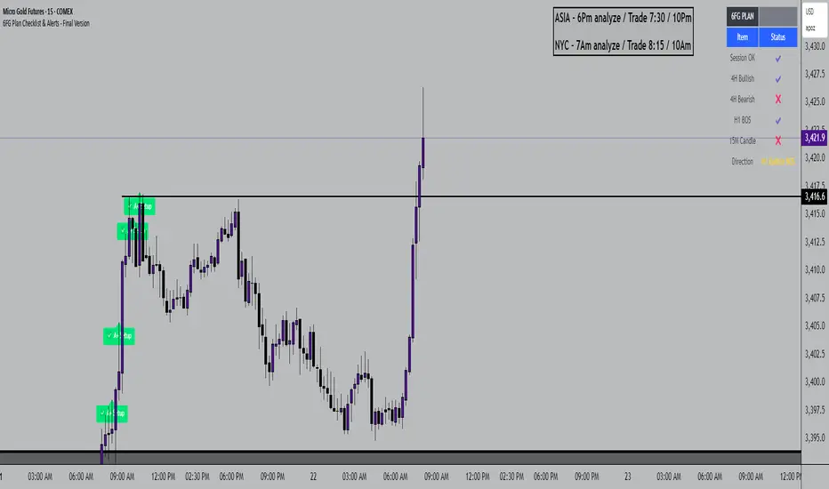
6FG Plan Checklist & Alerts - Final Version🧠 SCRIPT OVERVIEW: "6FG A+ SETUP - Simplified"
This script is designed to identify high-probability A+ trade setups in alignment with your personal 6FG trading plan, based on:
H1 Break of Structure (required)
4H trend confirmation
15M candle confirmation
Session filter
A+ Label & Visual Table Checklist
✅ KEY COMPONENTS
1. Toggle Inputs
These allow you to customize your view and filters without changing the code:
showSession: Only allow alerts inside Asian or NY sessions
show4hTrend: Include or ignore 4H directional bias
show15mConfirm: Include or ignore confirmation from 15M candles
showTable: Display checklist table on chart
showLabel: Display the “✅ A+” label on qualifying bars
2. Session Filter
Defines valid timeframes for trading (Asian or New York)
Helps avoid setups during low-liquidity hours
Controlled by showSession
3. 4H Trend (Confirmation Only)
Uses a 20-period SMA on 4H to detect general bias:
Bullish = Price above SMA
Bearish = Price below SMA
This trend is not mandatory for an alert if toggle is off
4. H1 Break of Structure (REQUIRED)
Looks at the highest high and lowest low of the last 10 candles on the 1H timeframe
Detects either:
Bullish BOS = Current close > highest high
Bearish BOS = Current close < lowest low
This is the core trigger for the A+ setup
If BOS doesn't happen, no entry is valid
5. 15M Confirmation Candles
(Optional - controlled by show15mConfirm)
Checks for one of three confirmation patterns:
Bullish Engulfing
Bearish Engulfing
Pin Bar
This adds confidence but can be toggled off
6. Entry Conditions (A+ Setup)
All the following must be true for entryOK = true:
✅ H1 BOS (required)
✅ Session is valid (if toggle is on)
✅ 15M confirmation pattern (if toggle is on)
✅ 4H trend (if toggle is on)
7. Visual Output
If entryOK = true:
✅ A green "A+" label appears below price
✅ A checklist table on the top-right shows:
Session status ✔️❌
4H bullish/bearish ✔️❌
H1 BOS ✔️❌
15M confirmation ✔️❌
Final Direction: Bullish / Bearish / —
A+ Setup: ✔️❌
8. Alerts
You will receive a TradingView alert when an A+ Setup is detected:
OBLibrary "OB"
The library is searching the OB
find_bull_ob(provided_OBs, low_1, high_1, settings_left_time, bar_closed, requested_close, requested_open, requested_low, WATCH_FROM_CANDLE_INDEX, WATCH_BACK_FROM_CANDLE_INDEX, PIVOT_EXTREMUM, GAP_REQUIREMENT)
Parameters:
provided_OBs (array type from maksym_hayovets/POITypes/6)
low_1 (float)
high_1 (float)
settings_left_time (int)
bar_closed (bool)
requested_close (float)
requested_open (float)
requested_low (float)
WATCH_FROM_CANDLE_INDEX (int)
WATCH_BACK_FROM_CANDLE_INDEX (int)
PIVOT_EXTREMUM (int)
GAP_REQUIREMENT (float)
find_bear_ob(provided_OBs, low_1, high_1, time_3, bar_closed, close_1, close_2, open_2, high_2, WICK_MULTIPLIER_SIZE, PIVOT_EXTREMUM)
Parameters:
provided_OBs (array type from maksym_hayovets/POITypes/6)
low_1 (float)
high_1 (float)
time_3 (int)
bar_closed (bool)
close_1 (float)
close_2 (float)
open_2 (float)
high_2 (float)
WICK_MULTIPLIER_SIZE (float)
PIVOT_EXTREMUM (int)

Supertrend Strategy (5m)📊 Strategy: Buy/Sell Based on EMA Crossover (5-Minute Timeframe)
📊 Стратегия: Buy/Sell по пересечению EMA (5 минут)

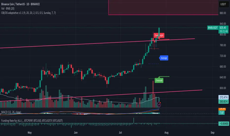
OB/OS adaptative v1.1# OB/OS Adaptative v1.1 - Multi-Timeframe Adaptive Overbought/Oversold Indicator
## Overview
The `tradingview_indicator_emas.pine` script is a sophisticated multi-timeframe indicator designed to identify dynamic overbought and oversold levels in financial markets. It combines EMA (Exponential Moving Average) crossovers and Bollinger Bands across monthly, weekly, and daily timeframes to create adaptive support and resistance levels that adjust to changing market conditions.
## Core Functionality
### Multi-Timeframe Analysis
The indicator analyzes three timeframes simultaneously:
- **Monthly (M)**: Long-term trend identification
- **Weekly (W)**: Intermediate-term trend identification
- **Daily (D)**: Short-term volatility measurement
### Technical Indicators Used
- **EMA 9 and EMA 20**: For trend identification and momentum assessment
- **Bollinger Bands (20-period)**: For volatility measurement and extreme level identification
- **Price action**: For confirmation of level validity and signal generation
## Key Features
### Adaptive Level Calculation
The indicator dynamically determines overbought and oversold levels based on market structure and trend bias:
#### Monthly Level Logic
- **Bullish Bias** (when monthly open > EMA20):
- Oversold = lower of EMA9 or EMA20
- Overbought = upper of EMA9 or Bollinger Upper Band
- **Bearish/Neutral Bias** (when monthly open ≤ EMA20):
- Oversold = Bollinger Lower Band
- Overbought = upper of EMA20 or EMA9
#### Weekly Level Logic
- **Bullish Bias** (when weekly open > EMA20):
- Oversold = lower of EMA9 or EMA20
- Overbought = Bollinger Upper Band
- **Bearish/Neutral Bias** (when weekly open ≤ EMA20):
- Oversold = Bollinger Lower Band
- Overbought = upper of EMA20 or EMA9
#### Daily Level Logic
- Simple Bollinger Bands:
- Oversold = Bollinger Lower Band
- Overbought = Bollinger Upper Band
### Final Level Determination
The indicator combines all three timeframes through a weighted averaging process:
1. Calculates initial values as the average of monthly, weekly, and daily levels
2. Ensures mathematical consistency by enforcing overbought_final ≥ oversold_final using min/max functions
3. Calculates a midpoint average level as the center of the range
### Visual Elements
- **Dynamic Lines**: Draws horizontal lines for current and previous period overbought, oversold, and average levels
- **Labels**: Places clear textual labels at the start of each period
- **Color Coding**:
- Red for overbought levels (resistance)
- Green for oversold levels (support)
- Blue for average levels (pivot point)
- **Transparency**: Previous period lines use semi-transparent colors to distinguish between current and historical levels
### Update Mechanism
- **Calculation Day**: User-defined day of the week (default: Monday)
- On the specified calculation day, the indicator:
- Updates all levels based on previous bar's data
- Draws new lines extending forward for a user-defined number of days
- Maintains previous period lines for comparison and trend analysis
- Automatically deletes and recreates lines to ensure clean visualization
### Proximity Detection
- Alerts when price approaches overbought/oversold levels (configurable distance in percentage)
- Helps identify potential reversal zones before actual crossovers occur
- Distance thresholds are user-configurable for both overbought and oversold conditions
### Alert Conditions
The indicator provides four distinct alert types:
1. **Cross below oversold**: Triggered when price crosses below the oversold level
2. **Cross above overbought**: Triggered when price crosses above the overbought level
3. **Near oversold**: Triggered when price approaches the oversold level within the configured distance
4. **Near overbought**: Triggered when price approaches the overbought level within the configured distance
### Debug Mode
When enabled, displays comprehensive debug information including:
- Current values for all levels (oversold, overbought, average)
- Timeframe-specific calculations and raw data points
- System status information (current day, calculation day, etc.)
- Lines existence and timing information
- Organized in multiple labels at different price levels to avoid overlap
## Configuration Parameters
| Parameter | Default Value | Description |
|---------|---------------|-------------|
| Short EMA (9) | 9 | Length for short-term EMA calculation |
| Long EMA (20) | 20 | Length for long-term EMA calculation |
| BB Length | 20 | Period for Bollinger Bands calculation |
| Std Dev | 2.0 | Standard deviation multiplier for Bollinger Bands |
| Distance to overbought (%) | 0.5 | Percentage threshold for "near overbought" alerts |
| Distance to oversold (%) | 0.5 | Percentage threshold for "near oversold" alerts |
| Calculation day | Monday | Day of week when levels are recalculated |
| Lookback days | 7 | Number of days to extend previous period lines backward |
| Forward days | 7 | Number of days to extend current period lines forward |
| Show Debug Labels | false | Toggle for comprehensive debug information display |
## Trading Applications
### Primary Use Cases
1. **Reversal Trading**: Identify potential reversal zones when price approaches overbought/oversold levels
2. **Trend Confirmation**: Use the adaptive nature of levels to confirm trend strength and direction
3. **Position Sizing**: Adjust position size based on distance from key levels
4. **Stop Placement**: Use opposite levels as dynamic stop-loss references
### Strategic Advantages
- **Adaptive Nature**: Levels adjust to changing market volatility and trend structure
- **Multi-Timeframe Confirmation**: Signals are validated across multiple timeframes
- **Visual Clarity**: Clear color-coded lines and labels enhance decision-making
- **Proactive Alerts**: "Near" conditions provide early warnings before crossovers
## Implementation Details
### Data Security
Uses `request.security()` function to fetch data from higher timeframes (monthly, weekly) while maintaining proper bar indexing with ` ` offset for open prices.
### Performance Optimization
- Uses `var` keyword to declare persistent variables that maintain state across bars
- Efficient line and label management with proper deletion before recreation
- Conditional execution of debug code to minimize performance impact
### Error Handling
- Comprehensive NA (not available) checks throughout the code
- Graceful degradation when data is unavailable for higher timeframes
- Mathematical safeguards to prevent invalid level calculations
## Conclusion
The OB/OS Adaptative v1.1 indicator represents a sophisticated approach to identifying market extremes by combining multiple technical analysis concepts. Its adaptive nature makes it particularly useful in trending markets where static levels may be less effective. The multi-timeframe approach provides a comprehensive view of market structure, while the visual elements and alert system enhance its practical utility for active traders.

Nifty Buy/Sell Signals with RSI & Fisheruy Signal when:
RSI crosses above 40 from below.
Fisher Transform crosses above its signal line (bullish crossover).
Sell Signal when:
RSI crosses below 60 from above.
Fisher Transform crosses below its signal line (bearish crossover).

MarketCapLibrary12Library "MarketCapLibrary12"
setMarketCapMap(m)
Parameters:
m (map)
getMarketCap(ticker)
Parameters:
ticker (string)

MarketCapLibrary11Library "MarketCapLibrary11"
setMarketCapMap(m)
Parameters:
m (map)
getMarketCap(ticker)
Parameters:
ticker (string)

15Min Volume x3 Spikeit show high power candels to conferm breakouts to hekp traders understand market better

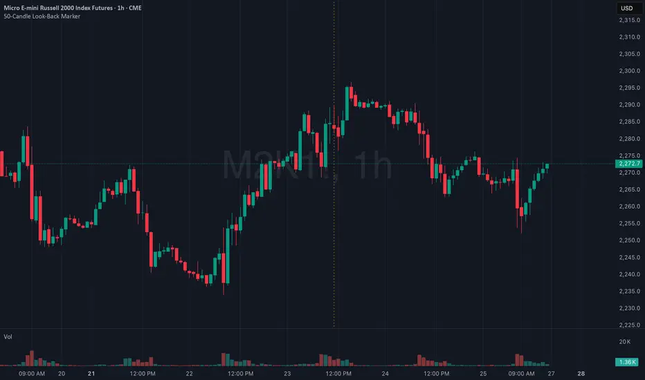
50-Candle Look-Back MarkerIt simply redraws one vertical dotted line that always sits exactly 50 bars behind the current bar, so you can check at a glance that any trend-line you draw has at least 50 candles of data to the right of it.
FVG + IFVG Gap (ULTRA) by Aditya NejeThis Indicator shows Fair Value Gap and Inverse Fair Value gaps

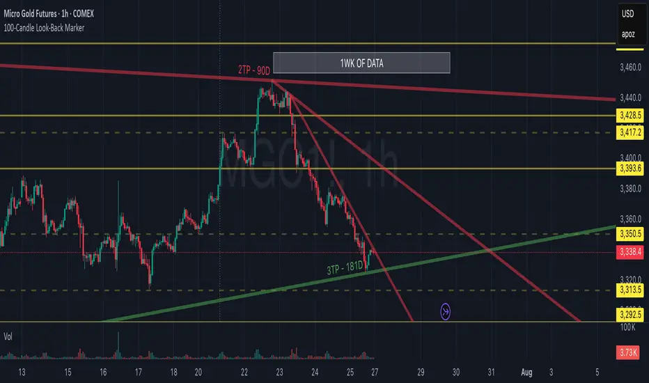
100-Candle Look-Back MarkerIt simply redraws one vertical dotted line that always sits exactly 100 bars behind the current bar, so you can check at a glance that any trend-line you draw has at least 100 candles of data to the right of it.
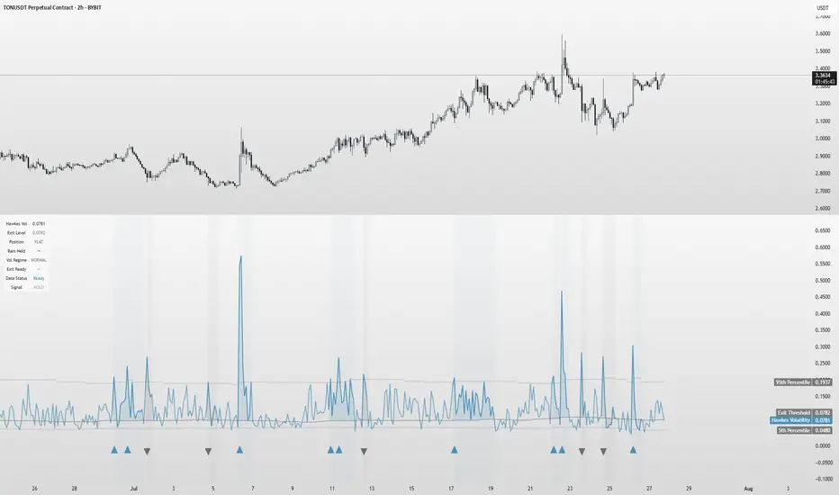
Hawkes Volatility Exit IndicatorOverview
The Hawkes Volatility Exit Indicator is a powerful tool designed to help traders capitalize on volatility breakouts and exit positions when momentum fades. Built on the Hawkes process, it models volatility clustering to identify optimal entry points after quiet periods and exit signals during volatility cooling. Designed to be helpful for swing traders and trend followers across markets like stocks, forex, and crypto.
Key Features Volatility-Based Entries: Detects breakouts when volatility spikes above the 95th percentile (adjustable) after quiet periods (below 5th percentile).
This indicator is probably better on exits than entries.
Smart Exit Signals: Triggers exits when volatility drops below a customizable threshold (default: 30th percentile) after a minimum hold period.
Hawkes Process: Uses a decay-based model (kappa) to capture volatility clustering, making it responsive to market dynamics.
Visual Clarity: Includes a volatility line, exit threshold, percentile bands, and intuitive markers (triangles for entries, X for exits).
Status Table: Displays real-time data on position (LONG/SHORT/FLAT), volatility regime (HIGH/LOW/NORMAL), bars held, and exit readiness.
Customizable Alerts: Set alerts for breakouts and exits to stay on top of trading opportunities.
How It Works Quiet Periods: Identifies low volatility (below 5th percentile) that often precede significant moves.
Breakout Entries: Signals bullish (triangle up) or bearish (triangle down) entries when volatility spikes post-quiet period.
Exit Signals: Suggests exiting when volatility cools below the exit threshold after a minimum hold (default: 3 bars).
Visuals & Table: Tracks volatility, position status, and signals via lines, shaded zones, and a detailed status table.
Settings
Hawkes Kappa (0.1): Adjusts volatility decay (lower = smoother, higher = more sensitive).
Volatility Lookback (168): Sets the period for percentile calculations.
ATR Periods (14): Normalizes volatility using Average True Range.
Breakout Threshold (95%): Volatility percentile for entries.
Exit Threshold (30%): Volatility percentile for exits.
Quiet Threshold (5%): Defines quiet periods.
Minimum Hold Bars (3): Ensures positions are held before exiting.
Alerts: Enable/disable breakout and exit alerts.
How to Use
Entries: Look for triangle markers (up for long, down for short) and confirm with the status table showing "ENTRY" and "LONG"/"SHORT."
Exits: Exit on X cross markers when the status table shows "EXIT" and "Exit Ready: YES."
Monitoring: Use the status table to track position, bars held, and volatility regime (HIGH/LOW/NORMAL).
Combine: Pair with price action, support/resistance, or other indicators for better context.
Tips : Adjust thresholds for your market: lower breakout thresholds for more signals, higher exit thresholds for earlier exits.
Test on your asset to ensure compatibility (best for markets with volatility clustering).
Use alerts to automate signal detection.
Limitations Requires sufficient data (default: 168 bars) for reliable signals. Check "Data Status" in the table.
Focuses on volatility, not price direction—combine with trend tools.
May lag slightly due to the smoothing nature of the Hawkes process.
Why Use It?
The Hawkes Volatility Exit Indicator offers a unique, data-driven approach to timing trades based on volatility dynamics. Its clear visuals, customizable settings, and real-time status table make it a valuable addition to any trader’s toolkit. Try it to catch breakouts and exit with precision!
This indicator is based on neurotrader888's python repo. All credit to him. All mistakes mine.
This conversion published for wider attention to the Hawkes method.
Weekly 8 EMA Horizontal Linethis will automatically track the WEEKLY 8EMA on your chart so you can know where the Weekly 8EMA is on lower timeframes
Fibonacci Range Detector ║ BullVision🔬 Overview
The Fibonacci Range Mapper is a dynamic technical tool designed to identify, track, and visualize price ranges using Fibonacci levels. Whether you're trading manually or prefer automated structure recognition, this indicator helps you contextualize market moves and locate key price zones with precision.
⚙️ Core Logic
🔍 Range Detection (Auto & Manual Modes)
In Auto mode, the indicator uses an advanced ZigZag system based on ATR or percentage thresholds to confirm market swings and construct Fibonacci-based ranges.
In Manual mode, traders can define their own swing low and high to generate precise custom ranges.
📐 Fibonacci Mapping
Each detected range is automatically plotted with key Fibonacci retracement levels — 0%, 25%, 50%, 75%, 100% — along with optional extensions (127.2% and 161.8%) to anticipate price continuations or reversals.
📋 Live Data Table
An integrated info panel dynamically displays crucial metrics:
• Range size
• Current price zone (Discount / Mid / Premium)
• Position within range (%)
• Distance to range extremes
• Range status (Pending or Confirmed)
🕰️ Historical Memory
Up to 20 past ranges can be stored and visualized simultaneously, helping traders recognize repeated price behaviors and contextual support/resistance levels.
🎨 Visual Highlights
Zones of interest (0–25% = Discount, 75–100% = Premium) are color-coded with custom transparency, and labels can be toggled for clarity. The current active range updates in real time as structure evolves.
🔧 User Customization
• Detection Method: Choose between ATR or % ZigZag for automated swing identification
• Confirmation Delay: Set how many bars to wait before confirming a new high
• Manual Overrides: Select exact price levels when you want full control
• Extensions & Labels: Toggle additional lines and info to suit your charting style
• Visual Table Position: Customize where the data table appears on screen
• Color Scheme: Define your own zone gradients for better visual interpretation
📈 Use Cases
This indicator is ideal for traders who want to:
• Identify value zones within local or macro price structures
• Plan trades around Fibonacci retracement and extension levels
• Detect shifts in market structure using an adaptive ZigZag logic
• Track recurring price ranges and historical reaction points
• Enhance technical confluence with clean, visual price mapping
⚠️ Important Notes
This tool is not a buy/sell signal generator — it is a visual framework for structure-based analysis.
Use it in conjunction with your existing strategy and risk management process.
Always confirm with broader context and multi-timeframe alignment.


Hypothesis TF Strategy EvaluationThis script provides a statistical evaluation framework for trend-following strategies by examining whether mean returns (measured here as 1-period Rate of Change, ROC) differ significantly across different price quantile groups.
Specifically, it:
Calculates rolling 25th (Q1) and 75th (Q3) percentile levels of price over a user-defined window.
Classifies returns into three groups based on whether price is above Q3, between Q1 and Q3, or below Q1.
Computes mean returns and sample sizes for each group.
Performs Welch's t-tests (which account for unequal variances) between groups to assess if their mean returns differ significantly.
Displays results in two tables:
Summary Table: Shows mean ROC and number of observations for each group.
Hypothesis Testing Table: Shows pairwise t-statistics with significance stars for 95% and 99% confidence levels.
Key Features
Rolling quantile calculations: Captures local price distributions dynamically.
Robust hypothesis testing: Welch's t-test allows for heteroskedasticity between groups.
Significance indicators: Easy visual interpretation with "*" (95%) and "**" (99%) significance levels.
Visual aids: Plots Q1 and Q3 levels on the price chart for intuitive understanding.
Extensible and transparent: Fully commented code that emphasizes the evaluation process rather than trading signals.
Important Notes
Not a trading strategy: This script is intended as a tool for research and validation, not as a standalone trading system.
Look-ahead bias caution: The calculation carefully avoids look-ahead bias by computing quantiles and ROC values only on past data at each point.
Users must ensure look-ahead bias is removed when applying this or similar methods, as look-ahead bias would artificially inflate performance and statistical significance.
The statistical tests rely on the assumption of independent samples, which might not fully hold in financial time series but still provide useful insights
Usage Suggestions
Use this evaluation framework to validate hypotheses about the behavior of returns under different price regimes.
Integrate with your strategy development workflow to test whether certain market conditions produce statistically distinct return distributions.
Example
In this example, the script was run with a quantile length of 20 bars and a lookback of 500 bars for ROC classification.
We consider a simple hypothetical "strategy":
Go long if the previous bar closed above Q3 the 75th percentile).
Go short if the previous bar closed below Q1 (the 25th percentile).
Stay in cash if the previous close was between Q1 and Q3.
The screenshot below demonstrates the results of this evaluation. Surprisingly, the "long" group shows a negative average return, while the "short" group has a positive average return, indicating mean reversion rather than trend following.
The hypothesis testing table confirms that the only statistically significant difference (at 95% or higher confidence) is between the above Q3 and below Q1 groups, suggesting a meaningful divergence in their return behavior.
This highlights how this framework can help validate or challenge intuitive assumptions about strategy performance through rigorous statistical testing.