DCA (ASAP) V0 PTTScript Name: DCA (ASAP) V0 PTT
Detailed Description:
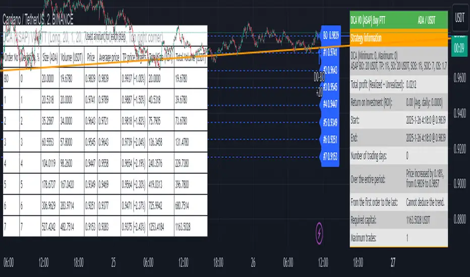
This script implements the Dollar-Cost Averaging (DCA) strategy, allowing you to automatically manage buy/sell orders safely and efficiently. Below are the key features of this script:
1. Purpose and Operation:
o Supports both Long and Short trading modes.
o Designed to optimize profitability using the DCA method, where Safety Orders are triggered when the price moves against the predicted direction.
o Helps users maintain their Target Profit in various market conditions.
2. Main Features:
o Automatic Order Placement: The initial Base Order is opened as soon as no active order exists.
o Safety Order Management: Safety Orders are automatically placed when the price moves against the initial order. The volume and distance of these orders are customizable.
o Order Closing: Orders are closed upon reaching the Target Profit, accounting for transaction fees.
o Detailed Information Display: Displays open orders, trading statistics, and performance metrics directly on the chart.
3. Customizable Parameters:
o Base Order Size: The size of the initial order.
o Target Profit (%): Target profit as a percentage of the total order volume.
o Safety Order Size: The size of each Safety Order.
o Price Deviation (%): The percentage distance between consecutive Safety Orders.
o Safety Order Volume Scale: The scaling factor for increasing the volume of subsequent Safety Orders.
o Max Safety Orders: The maximum number of Safety Orders allowed per deal.
4. Unique Features:
o Backtest Range Support: Enables you to limit backtesting to a specific time range of interest.
o Comprehensive Statistics: Displays detailed tables including open trades, pending orders, ROI, trading days, and realized profit.
o Integrated Trading Fees: Includes transaction fees in profit calculations for precise results.
5. Usage Instructions:
o Select the trading mode (Long or Short) from the "Strategy" input.
o Customize parameters such as Base Order, Safety Order, and Target Profit according to your requirements and the asset being traded.
o Monitor the performance of the strategy through the displayed information tables.
Notes:
• This script does not disclose detailed calculation logic but provides an overview of the concepts and usage.
• Designed for trading on exchanges that support margin or spot trading.
Pine utilities
Outside Bar Strategy % (Alessio)Outside Bar Strategy %
This strategy is based on identifying Outside Bars, which occur when the current bar's high is higher than the previous bar's high and its low is lower than the previous bar's low. The strategy enters trades in the direction of the Outside Bar, offering a powerful way to capture price moves following a strong price expansion.
Key Features:
Long and Short Entries: The strategy enters a Long trade when the Outside Bar closes bullish (current close > open), and a Short trade when the Outside Bar closes bearish (current close < open).
Customizable Entry Levels: The entry point is calculated based on a customizable percentage of the Outside Bar's range, allowing flexibility for traders to fine-tune their entries at 50% or 70% of the bar's range.
Stop Loss (SL) and Take Profit (TP):
Stop Loss (SL) is automatically placed at the Outside Bar's low for Long trades and at its high for Short trades.
Take Profit (TP) is calculated as a percentage of the Outside Bar's range, with customizable settings for take-profit levels.
Visual Indicators:
Entry, Stop Loss, and Take Profit levels are plotted as lines on the chart, with customizable colors and widths for easy identification.
Labels are placed on the chart to indicate whether the trade is Long or Short, positioned above or below the Outside Bar's candlestick.
Alerts: Users can enable alerts to receive notifications when a trade is triggered, including details such as entry points and stop loss levels.
Strategy Parameters:
Entry Percentage: Set the entry level as a percentage of the Outside Bar's range (e.g., 50%, 70%).
Take Profit Percentage: Customize the Take Profit level as a percentage of the Outside Bar's range.
Customizable Colors and Line Widths: Adjust the colors and thickness of the entry, stop loss, and take profit lines to fit your preferences.
Alerts: Enable alerts to be notified when a trade is executed or when the entry level is reached.
This strategy is ideal for traders who want to capitalize on significant price moves after a breakout, with clear risk management through Stop Loss and Take Profit levels. The customizable features make it suitable for various market conditions and trading styles.

TDGS Dynamic Grid Trading Strategy [CoinFxPro]Advanced Dynamic Grid Trading Strategy
Logic and Working Principle:
This strategy uses a dynamic grid system to support both long and short trades. Grid trading aims to capitalize on price fluctuations within a predefined range by executing buy and sell orders systematically. The system calculates grid levels based on a base price and dynamically trades within these levels.
Grid Levels:
Grid levels are calculated based on the initial price and the user-defined grid spacing percentage.
Long Mode: Buys when the price decreases and sells when the price increases.
Short Mode: Sells when the price increases and buys when the price decreases.
Grid Updates:
Grid levels are recalculated based on the market price when the price moves by a user-defined update percentage.
For example;
In Long mode, when the price shows an upward trend, that is, when it rises by the Grid Update Percentage specified by the user, Grid levels are recreated and trades are made according to the new grid levels. While the price and grid levels are updated according to the new price, the Stop level is also updated upwards and the stop is followed with the TrailingStop logic.
In short mode, the same system operates with reverse logic. In other words, as prices decrease downwards, the grids are updated downwards when the Grid update percentage determined by the user decreases. The stop level is also updated accordingly.
The difference of the strategy from other Gridbots is that the grid levels are automatically updated and the levels are recreated with the price percentage difference determined by the user. Old levels can be tracked on the chart.
As the price updates, the self-updating grid levels are updated upwards in long mode and downwards in short mode.
The number of buying lots and selling lots are separated, allowing both trading within the position and the opportunity to collect lots and increase the position.
When trading with the grid trading logic, when buying and selling between grids, there is no repeated purchase at the same level unless there is a sale at the upper grid level. In this way, each level will be traded within itself.
For example, in a long condition, when the price is going up, after deducting the selling lot from the buying lot at each level, the remaining lots will be collected while the price is going up and an opportunity will be provided from the price rise.
Different preferences have been added to the profit taking conditions, allowing the robot to continue or stop after profit taking, if desired.
The system, which acts entirely according to user parameters, constantly updates itself as long as it moves in the direction determined by itself, and in these conditions, transactions are carried out according to profit or stop conditions.
Parameters:
Grid Parameters:
Settings such as buy lot size, sell lot size, grid count, and grid spacing percentage allow flexibility and customization.
Risk Management:
Stop loss (%) and take profit (%) levels help limit potential losses and secure profits at predefined thresholds.
Objective:
The goal of this strategy is to systematically capitalize on market price fluctuations through automated grid trading. This method is particularly effective in volatile markets where the price oscillates within a specific range.
The strategy works with a complete algorithm logic, and in appropriate instruments (especially instruments with depth and transaction volume should be preferred), buying and selling transactions are made according to the parameters determined at the beginning, and if the conditions go beyond the conditions, the stop is made, and when the profit taking conditions are met, it takes profit and prices according to the determined value. When it is updated, the values are updated again and the parameter works algorithmically.
Risk Management Recommendations:
Initial Capital: Grid trading involves frequent transactions, so sufficient initial capital is essential.
Stop Loss: Always set stop loss levels to prevent significant losses.
Grid Count and Spacing: A higher number of grids provides more trading opportunities but using grids that are too close may increase transaction costs due to small price movements.
First of all, it is important for risk management that you choose instruments that have depth and high transaction volume.
Strategy results may differ as a result of the parameters entered. Therefore, before trading in your real account, it is recommended that you start real transactions after backtesting with different parameters.
If you are stuck on something, you can mention it in the comments.

Fibonacci Retracement Strategy for CryptoThe Enhanced Fibonacci Retracement Strategy is designed to help traders capitalize on key Fibonacci levels for both long and short trades. This script automatically identifies significant swing highs and lows within a customizable lookback period and dynamically plots Fibonacci retracement levels (0%, 23.6%, 38.2%, 50%, 61.8%, 78.6%, and 100%) as support and resistance levels.
Key Features:
Automatic Fibonacci Levels:
The script identifies the highest high and lowest low over a user-defined lookback period to calculate Fibonacci retracement levels.
Dual-Directional Trading:
Long Trades: Triggered when the price crosses above the 61.8% retracement level, anticipating a reversal.
Short Trades: Triggered when the price crosses below the 38.2% retracement level, capturing potential downward movement.
Compact Line Option:
Users can toggle "Compact Fibonacci Lines" to reduce visual clutter on the chart, making the lines shorter and easier to interpret.
Dynamic Alerts:
Alerts are embedded directly into the strategy logic for entry and exit points.
Long Entry: Triggered when the price bounces above the 61.8% level.
Long Exit: Triggered when the price reaches the 23.6% level.
Short Entry: Triggered when the price crosses below the 38.2% level.
Short Exit: Triggered when the price reaches the 78.6% level.
Clear Visualization:
Fibonacci levels are plotted with distinct colors and dashed lines (optional compact view),
providing traders with clear and actionable levels to make decisions.
Inputs:
Lookback Period: Number of candles to calculate swing highs and lows.
Plot Fibonacci Levels: Toggle to enable/disable plotting levels.
Compact Fibonacci Lines: Reduce the length of Fibonacci lines for a cleaner chart.
How It Works:
The strategy identifies a high-low range within the lookback period.
Fibonacci levels are calculated based on the range and plotted on the chart.
Long Trade Example:
Enter when the price crosses above the 61.8% level.
Exit when the price reaches the 23.6% level.
Short Trade Example:
Enter when the price crosses below the 38.2% level.
Exit when the price reaches the 78.6% level.
Best Use Cases:
Trending Markets: Use retracements to time entries in the direction of the trend.
Range-Bound Markets: Identify and trade reversals near key Fibonacci levels.
Important Notes:
This strategy is not financial advice and should be backtested thoroughly before live trading.
Risk management is crucial! Consider using stop-loss orders for protection.
Customize inputs to suit your preferred timeframe and trading style.

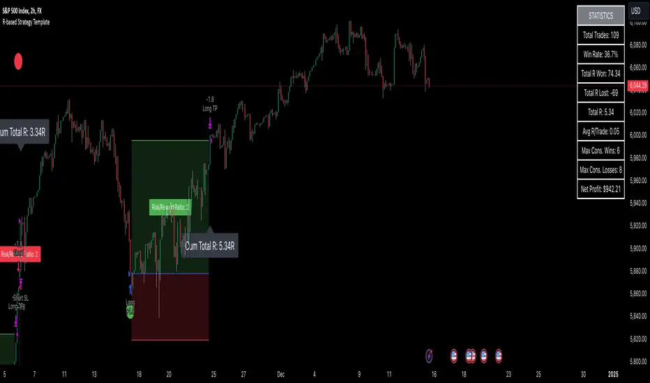
R-based Strategy Template [Daveatt]Have you ever wondered how to properly track your trading performance based on risk rather than just profits?
This template solves that problem by implementing R-multiple tracking directly in TradingView's strategy tester.
This script is a tool that you must update with your own trading entry logic.
Quick notes
Before we dive in, I want to be clear: this is a template focused on R-multiple calculation and visualization.
I'm using a basic RSI strategy with dummy values just to demonstrate how the R tracking works. The actual trading signals aren't important here - you should replace them with your own strategy logic.
R multiple logic
Let's talk about what R-multiple means in practice.
Think of R as your initial risk per trade.
For instance, if you have a $10,000 account and you're risking 1% per trade, your 1R would be $100.
A trade that makes twice your risk would be +2R ($200), while hitting your stop loss would be -1R (-$100).
This way of measuring makes it much easier to evaluate your strategy's performance regardless of account size.
Whenever the SL is hit, we lose -1R
Proof showing the strategy tester whenever the SL is hit: i.imgur.com
The magic happens in how we calculate position sizes.
The script automatically determines the right position size to risk exactly your specified percentage on each trade.
This is done through a simple but powerful calculation:
risk_amount = (strategy.equity * (risk_per_trade_percent / 100))
sl_distance = math.abs(entry_price - sl_price)
position_size = risk_amount / (sl_distance * syminfo.pointvalue)
Limitations with lower timeframe gaps
This ensures that if your stop loss gets hit, you'll lose exactly the amount you intended to risk. No more, no less.
Well, could be more or less actually ... let's assume you're trading futures on a 15-minute chart but in the 1-minute chart there is a gap ... then your 15 minute SL won't get filled and you'll likely to not lose exactly -1R
This is annoying but it can't be fixed - and that's how trading works anyway.
Features
The template gives you flexibility in how you set your stop losses. You can use fixed points, ATR-based stops, percentage-based stops, or even tick-based stops.
Regardless of which method you choose, the position sizing will automatically adjust to maintain your desired risk per trade.
To help you track performance, I've added a comprehensive statistics table in the top right corner of your chart.
It shows you everything you need to know about your strategy's performance in terms of R-multiples: how many R you've won or lost, your win rate, average R per trade, and even your longest winning and losing streaks.
Happy trading!
And remember, measuring your performance in R-multiples is one of the most classical ways to evaluate and improve your trading strategies.
Daveatt
FXC NQ Opening Range Breakout Strategy V2.4Mechanical Strategy that trades breakouts on NQ futures on the 15min timeframe during the NYSE session. It's designed to manage Apex and Top Step accounts with the lowest risk possible.
Risk Disclaimer:
Past results as well as strategy tester reports do not indicate future performance. Guarantees do not exist in trading. By using this strategy you risk losing all your money.
Important:
It only trades on Monday, Wednesday and Friday and takes usually only 1 trade per trading day.
It works on the 15min timeframe only.
The settings are optimised already for NQ but feel free to change them.
How it works:
Every selected trading day it measures the range of the first 15min candle after the NYSE open. As soon as price closes above on the 15min timeframe, it will trade the breakout targeting a set risk to reward ratio. SL on the opposite side of the range. It will trail the SL after a set amount of points and uses a buffer of the set amount of points to trail it.
Settings:
Opening Range Time : This is the time of the day in hours and minutes when the strategy starts looking for trades. It's in the EST/ NY Timezone and set to 9:30-09:45 by default
because that's the NYSE open.
Session Time : This is the time of the day in hours and minutes until the strategy trades. It's in the EST/ NY Timezone and set to 09:45-14:45 by default.
because that's what gave the best results in backtesting. Open trades will get closed automatically once the end of the session is reached. No matter if win or loss. This is just to prevent holding positions over night.
Session Border This setting is to select the border color in which the session box will be plotted.
Opening Range Box This setting is to select the fill color of the opening range box.
Opening Range Border This setting is to select the border color of the session box.
Trade Timeframe This setting determines on which timeframe candle has to close outside the opening range box in order to take a trade. It's set to 15min by default because this is what worked by far the best in backtests and live trading.
Stop Loss Buffer in Points: This is simply the buffer in points that is added to the SL for safety reasons. If you have it on 0, the SL will be at the exact price of the opposite side of the range. By default it's set to 0 pips because this is what delivered the best results in backtests.
Profit Target Factor: This is simply the total SL size in points multiplied by x.
Example: If you put 2, you get a 1:2 Risk to Reward Ratio. By Default it's set to 4 because this gave the best results in backtests, because trades always get closed either by trailing SL or because the end of the session is reached.
Use Trailing Stop Loss: This setting is to enable/ disable the trailing stop loss. It's enabled by default because this is a fundamental part of the strategy.
Trailing Stop Buffer: This setting determines after how many points in profit the trailing SL will be activated.
Risk Type: You can chose either between Fixed USD Amount, Risk per Trade in % or Fixed Contract Size. By default it's set to fixed contract size.
Risk Amount (USD or Contracts): This setting is to set how many USD or how many contracts you want to risk per trade. Make sure to check which risk type you have selected before you chose the risk amount.
Use Limit Orders If enabled, the strategy will place a pending order x points from the current price, instead of a market order. Limit orders are enabled by default for a better performance. Important: It doesn't actually place a limit order. The strategy will just wait for a pullback and then enter with a market order. It's more like a hidden limit order.
Limit Order Distance (points): If you have limit orders enabled, this setting determines how many points from the current price the limit order will be placed.
Trading Days: These checkboxes are to select on which week days the strategy has to trade. Thursday is disabled by default because backtests have shown that Thursday is the least profitable day
Backtest Settings:
For the backtest the commissions ere set to 0.35 USD per mini contract which is the highest amount Tradeovate charges. Margin was not accounted for because typically on Apex accounts you can use way more contracts than you need for the extremely low max drawdown. Margin would be important on personal accounts but even there typically it's not an issue at all especially because this strategy runs on the 15min timeframe so it won't use a lot of contracts anyways.
What makes it unique:
This script is unique because it's designed to be used on Apex and Top Step accounts with extremely strict drawdown rules.
The strategy is optimised to be traded with a fixed contract size instead of using % risk. The reason for that is that the drawdown rules of these Futures Prop Accounts are very strict and the fact that the smallest trade-able contract size is 1.
Why the source code is hidden:
The source code is hidden because I invested a lot of time and money into developing this strategy and optimising it with paid 3rd party software. Also since I use it myself on my Apex accounts and prop firms don't allow copy trading I don't want it to be used by too many traders.
Liquid Pours XtremeStrategy Description: Liquid Pours Xtreme
The Liquid Pours Xtreme is an innovative trading strategy that combines the analysis of specific time-based patterns with price comparisons to identify potential opportunities in the forex market. Designed for traders seeking a structured methodology based on clear rules, this strategy offers integration with Telegram for real-time alerts and provides visual tools to enhance trade management.
Key Features:
Analysis of Specific Time Patterns: The strategy captures and compares closing prices at two key moments during the trading day, identifying recurring patterns that may indicate future market movements.
Dynamic SL and TP Levels Implementation: Utilizes tick-based calculations to set Stop-Loss and Take-Profit levels, adapting to the current market volatility.
Advanced Telegram Integration: Provides detailed alerts including information such as the asset, signal time, entry price, and SL/TP levels, facilitating real-time decision-making.
Complete Customization: Allows users to adjust key parameters, including operation schedules, weekdays, and visual settings, adapting to different trading styles.
Enhanced Chart Visualization: Includes visual elements like candle color changes based on signal state, event markers, and halos to highlight important moments.
Default Strategy Properties: Specific configuration for optimal risk management and simulation.
How the Strategy Works
Capturing Prices at Key Moments:
- The strategy records the closing price at two user-defined specific times. These times typically correspond to periods of high market volatility, such as the opening of the European session and the US pre-market.
- Rationale: Volatility and trading volume usually increase during these times, presenting opportunities for significant price movements.
Generating Signals Based on Price Comparison:
- Buy Signal: If the second closing price is lower than the first, it indicates possible accumulation and is interpreted as a bullish signal.
- Sell Signal: If the second closing price is higher than the first, it suggests possible distribution and is interpreted as a bearish signal.
- Signals are only generated on selected trading days, allowing you to avoid days with lower liquidity or higher risk.
Calculating Dynamic SL and TP Levels:
- Stop-Loss (SL) and Take-Profit (TP) levels are calculated based on the entry price and a user-defined number of ticks, adapting to market volatility.
- The strategy offers the option to base these levels on the close of the signal candle or the open of the next candle, providing flexibility according to the trader's preference.
- SL and TP boxes are drawn on the chart for visual reference, facilitating trade management.
Automatic Execution and Alerts:
- Upon signal generation, the strategy automatically executes a market order (buy or sell).
- Sends a detailed alert to your Telegram channel, including essential information for quick decision-making.
Visual Elements:
- Colors candles based on the signal state: buy, sell, or neutral, allowing for quick trend identification.
- Provides a smooth color transition between signal states and uses markers and halos to highlight important events and signals on the chart.
Trade Management:
- Manages open trades with automatic exit conditions based on the established SL and TP levels.
- Includes mechanisms to prevent exceeding TradingView's limitations on boxes and labels, ensuring optimal script performance.
Originality and utility:
- This strategy incorporates a unique approach focusing on specific time patterns and their relationship to institutional activity in the market.
How to Use the Strategy
Add the Script to the Chart:
- Go to the indicators menu in TradingView.
- Search for " Liquid Pours Xtreme " and add it to your chart.
Set Up Telegram Alerts:
- Enter your Telegram Chat ID in the script parameters to receive alerts.
- Customize the Buy and Sell alert messages as desired.
Configure Time Patterns:
- Set the hours and minutes for the two times you want to compare closing prices, aligning them with relevant market sessions or events.
Set SL and TP Parameters:
- Define the number of ticks for the Stop-Loss and Take-Profit levels, adapting them to the asset you're trading and your risk tolerance.
- Choose the basis for SL and TP calculation (close of the signal candle or open of the next candle).
Select Trading Days:
- Enable or disable trading on specific days of the week, allowing you to avoid days with lower activity or unexpected volatility.
Customize Visual Elements:
- Adjust the colors and styles of visual elements to enhance readability and suit your personal preferences.
Monitor the Strategy:
- Observe the chart for signals and use Telegram alerts to stay informed of new opportunities, even when you're not at your terminal.
Testing and Optimization:
- Use TradingView's backtesting features to evaluate the historical performance of the strategy with different parameters.
- Adjust and optimize the parameters based on the results and your own analysis.
Adjust the Strategy Properties:
- Ensure that the strategy properties (order size, commission, slippage) are aligned with your trading account and platform to obtain realistic results.
Strategy Properties (Important)
This script backtest is conducted on M30 EURUSD , using the following backtesting properties:
Initial Capital: $10,000
Order Size: 50,000 Contracts (equivalent to 0.5% of the capital)
Commission: $0.20 per order
Slippage: 1 tick
Pyramiding: 1 order
Verify Price for Limit Orders: 0 ticks
Recalculate on Order Execution: Enabled
Recalculate on Every Tick: Enabled
Recalculate After Order Filled: Enabled
Bar Magnifier for Backtesting Precision: Enabled
We use these properties to ensure a realistic preview of the backtesting system. Note that default properties may vary for different reasons:
- Order Size: It is essential to calculate the contract size according to the traded asset and desired risk level.
- Commission and Slippage: These costs can vary depending on the market and instrument; there is no default value that might return realistic results.
We strongly recommend all users adjust the Properties within the script settings to align with their accounts and trading platforms to ensure the results from the strategies are realistic.
Backtesting Results:
- Net Profit: $4,037.50 (40.37%)
- Total Closed Trades : 292
- Profitability Percentage: 26.71%
- Profit Factor: 1.369
- Max Drawdown: $769.30 (6.28%)
- Average Trade: $13.83 (0.03%)
- Average Bars in Trades: 11
These results were obtained under the mentioned conditions and properties, providing an overview of the strategy's historical performance.
Interpreting Results:
- The strategy has demonstrated profitability in the analyzed period, although with a win rate of 26.71%, indicating that success relies on a favorable risk-reward ratio.
- The profit factor of 1.369 suggests that total gains exceed total losses by that proportion.
- It is crucial to consider the maximum drawdown of 6.28% when evaluating the strategy's suitability to your risk tolerance.
Risk Warning:
Trading leveraged financial instruments carries a high level of risk and may not be suitable for all investors. Before deciding to trade, you should carefully consider your investment objectives, level of experience, and risk tolerance. Past performance does not guarantee future results. It is essential to conduct additional testing and adjust the strategy according to your needs.
---
What Makes This Strategy Original?
Time-Based Pattern Approach: Unlike conventional strategies, this strategy focuses on identifying time patterns that reflect institutional activity and macroeconomic events that can influence the market.
Advanced Technological Integration: The combination of automatic execution and customized alerts via Telegram provides an efficient and modern tool for active traders.
Customization and Adaptability: The wide range of adjustable parameters allows the strategy to be tailored to different assets, time zones, and trading styles.
Enhanced Visual Tools: Incorporated visual elements facilitate quick market interpretation and informed decision-making.
Additional Considerations
Continuous Testing and Optimization: Users are encouraged to perform additional backtesting and optimize parameters according to their own observations and requirements.
Complementary Analysis: Use this strategy in conjunction with other indicators and fundamental analysis to reinforce decision-making.
Rigorous Risk Management: Ensure that SL and TP levels, as well as position sizing, align with your risk management plan.
Updates and Support: I am committed to providing updates and improvements based on community feedback. For inquiries or suggestions, feel free to contact me.
---
Example Configuration
Assuming you want to use the strategy with the following parameters:
Telegram Chat ID: Your unique Telegram Chat ID
First Time (Hour:Minute): 6:30
Second Time (Hour:Minute): 7:30
SL Ticks: 100
TP Ticks: 400
SL and TP Basis: Close of the Signal Candle
Trading Days: Tuesday, Wednesday, Thursday
Simulated Initial Capital: $10,000
Risk per Trade in Simulation: $50 (-0.5% of capital)
Slippage and Commissions in Simulation: 1 tick of slippage and $0.20 commission per trade
---
Conclusion
The Liquid Pours Xtreme strategy offers an innovative approach by combining specific time analysis with robust risk management and modern technological tools. Its original and adaptable design makes it valuable for traders looking to diversify their methods and capitalize on opportunities based on less conventional patterns.
Ready for immediate implementation in TradingView, this strategy can enrich your trading arsenal and contribute to a more informed and structured approach to your operations.
---
Final Disclaimer:
Financial markets are volatile and can present significant risks. This strategy should be used as part of a comprehensive trading approach and does not guarantee positive results. It is always advisable to consult with a professional financial advisor before making investment decisions.
---

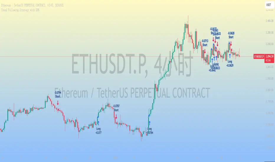
Trend Following Strategy with KNN
### 1. Strategy Features
This strategy combines the K-Nearest Neighbors (KNN) algorithm with a trend-following strategy to predict future price movements by analyzing historical price data. Here are the main features of the strategy:
1. **Dynamic Parameter Adjustment**: Uses the KNN algorithm to dynamically adjust parameters of the trend-following strategy, such as moving average length and channel length, to adapt to market changes.
2. **Trend Following**: Captures market trends using moving averages and price channels to generate buy and sell signals.
3. **Multi-Factor Analysis**: Combines the KNN algorithm with moving averages to comprehensively analyze the impact of multiple factors, improving the accuracy of trading signals.
4. **High Adaptability**: Automatically adjusts parameters using the KNN algorithm, allowing the strategy to adapt to different market environments and asset types.
### 2. Simple Introduction to the KNN Algorithm
The K-Nearest Neighbors (KNN) algorithm is a simple and intuitive machine learning algorithm primarily used for classification and regression problems. Here are the basic concepts of the KNN algorithm:
1. **Non-Parametric Model**: KNN is a non-parametric algorithm, meaning it does not make any assumptions about the data distribution. Instead, it directly uses training data for predictions.
2. **Instance-Based Learning**: KNN is an instance-based learning method that uses training data directly for predictions, rather than generating a model through a training process.
3. **Distance Metrics**: The core of the KNN algorithm is calculating the distance between data points. Common distance metrics include Euclidean distance, Manhattan distance, and Minkowski distance.
4. **Neighbor Selection**: For each test data point, the KNN algorithm finds the K nearest neighbors in the training dataset.
5. **Classification and Regression**: In classification problems, KNN determines the class of a test data point through a voting mechanism. In regression problems, KNN predicts the value of a test data point by calculating the average of the K nearest neighbors.
### 3. Applications of the KNN Algorithm in Quantitative Trading Strategies
The KNN algorithm can be applied to various quantitative trading strategies. Here are some common use cases:
1. **Trend-Following Strategies**: KNN can be used to identify market trends, helping traders capture the beginning and end of trends.
2. **Mean Reversion Strategies**: In mean reversion strategies, KNN can be used to identify price deviations from the mean.
3. **Arbitrage Strategies**: In arbitrage strategies, KNN can be used to identify price discrepancies between different markets or assets.
4. **High-Frequency Trading Strategies**: In high-frequency trading strategies, KNN can be used to quickly identify market anomalies, such as price spikes or volume anomalies.
5. **Event-Driven Strategies**: In event-driven strategies, KNN can be used to identify the impact of market events.
6. **Multi-Factor Strategies**: In multi-factor strategies, KNN can be used to comprehensively analyze the impact of multiple factors.
### 4. Final Considerations
1. **Computational Efficiency**: The KNN algorithm may face computational efficiency issues with large datasets, especially in real-time trading. Optimize the code to reduce access to historical data and improve computational efficiency.
2. **Parameter Selection**: The choice of K value significantly affects the performance of the KNN algorithm. Use cross-validation or other methods to select the optimal K value.
3. **Data Standardization**: KNN is sensitive to data standardization and feature selection. Standardize the data to ensure equal weighting of different features.
4. **Noisy Data**: KNN is sensitive to noisy data, which can lead to overfitting. Preprocess the data to remove noise.
5. **Market Environment**: The effectiveness of the KNN algorithm may be influenced by market conditions. Combine it with other technical indicators and fundamental analysis to enhance the robustness of the strategy.
FTMO Rules MonitorFTMO Rules Monitor: Stay on Track with Your FTMO Challenge Goals
TLDR; You can test with this template whether your strategy for one asset would pass the FTMO challenges step 1 then step 2, then with real money conditions.
Passing a prop firm challenge is ... challenging.
I believe a toolkit allowing to test in minutes whether a strategy would have passed a prop firm challenge in the past could be very powerful.
The FTMO Rules Monitor is designed to help you stay within FTMO’s strict risk management guidelines directly on your chart. Whether you’re aiming for the $10,000 or the $200,000 account challenge, this tool provides real-time tracking of your performance against FTMO’s rules to ensure you don’t accidentally breach any limits.
NOTES
The connected indicator for this post doesn't matter.
It's just a dummy double supertrends (see below)
The strategy results for this script post does not matter as I'm posting a FTMO rules template on which you can connect any indicator/strategy.
//@version=5
indicator("Supertrends", overlay=true)
// Supertrend 1 Parameters
var string ST1 = "Supertrend 1 Settings"
st1_atrPeriod = input.int(10, "ATR Period", minval=1, maxval=50, group=ST1)
st1_factor = input.float(2, "Factor", minval=0.5, maxval=10, step=0.5, group=ST1)
// Supertrend 2 Parameters
var string ST2 = "Supertrend 2 Settings"
st2_atrPeriod = input.int(14, "ATR Period", minval=1, maxval=50, group=ST2)
st2_factor = input.float(3, "Factor", minval=0.5, maxval=10, step=0.5, group=ST2)
// Calculate Supertrends
= ta.supertrend(st1_factor, st1_atrPeriod)
= ta.supertrend(st2_factor, st2_atrPeriod)
// Entry conditions
longCondition = direction1 == -1 and direction2 == -1 and direction1 == 1
shortCondition = direction1 == 1 and direction2 == 1 and direction1 == -1
// Optional: Plot Supertrends
plot(supertrend1, "Supertrend 1", color = direction1 == -1 ? color.green : color.red, linewidth=3)
plot(supertrend2, "Supertrend 2", color = direction2 == -1 ? color.lime : color.maroon, linewidth=3)
plotshape(series=longCondition, location=location.belowbar, color=color.green, style=shape.triangleup, title="Long")
plotshape(series=shortCondition, location=location.abovebar, color=color.red, style=shape.triangledown, title="Short")
signal = longCondition ? 1 : shortCondition ? -1 : na
plot(signal, "Signal", display = display.data_window)
To connect your indicator to this FTMO rules monitor template, please update it as follow
Create a signal variable to store 1 for the long/buy signal or -1 for the short/sell signal
Plot it in the display.data_window panel so that it doesn't clutter your chart
signal = longCondition ? 1 : shortCondition ? -1 : na
plot(signal, "Signal", display = display.data_window)
In the FTMO Rules Monitor template, I'm capturing this external signal with this input.source variable
entry_connector = input.source(close, "Entry Connector", group="Entry Connector")
longCondition = entry_connector == 1
shortCondition = entry_connector == -1
🔶 USAGE
This indicator displays essential FTMO Challenge rules and tracks your progress toward meeting each one. Here’s what’s monitored:
Max Daily Loss
• 10k Account: $500
• 25k Account: $1,250
• 50k Account: $2,500
• 100k Account: $5,000
• 200k Account: $10,000
Max Total Loss
• 10k Account: $1,000
• 25k Account: $2,500
• 50k Account: $5,000
• 100k Account: $10,000
• 200k Account: $20,000
Profit Target
• 10k Account: $1,000
• 25k Account: $2,500
• 50k Account: $5,000
• 100k Account: $10,000
• 200k Account: $20,000
Minimum Trading Days: 4 consecutive days for all account sizes
🔹 Key Features
1. Real-Time Compliance Check
The FTMO Rules Monitor keeps track of your daily and total losses, profit targets, and trading days. Each metric updates in real-time, giving you peace of mind that you’re within FTMO’s rules.
2. Color-Coded Visual Feedback
Each rule’s status is shown clearly with a ✓ for compliance or ✗ if the limit is breached. When a rule is broken, the indicator highlights it in red, so there’s no confusion.
3. Completion Notification
Once all FTMO requirements are met, the indicator closes all open positions and displays a celebratory message on your chart, letting you know you’ve successfully completed the challenge.
4. Easy-to-Read Table
A table on your chart provides an overview of each rule, your target, current performance, and whether you’re meeting each goal. The table adjusts its color scheme based on your chart settings for optimal visibility.
5. Dynamic Position Sizing
Integrated ATR-based position sizing helps you manage risk and avoid large drawdowns, ensuring each trade aligns with FTMO’s risk management principles.
Daveatt

TrendGuard Scalper: SSL + Hama Candle with Consolidation ZonesThis TradingView script brings a powerful scalping strategy that combines the SSL Channel and Hama Candles indicators with a special twist—consolidation detection. Designed for traders looking for consistency in various markets like crypto, forex, and stocks, this strategy highlights clear trend signals, risk management, and helps filter out risky trades during consolidation periods.
Why Use This Strategy?
Clear Trend Detection:
With the SSL Channel, you’ll know exactly when the market is in an uptrend (green) or downtrend (red), giving you straightforward entry points.
Short-Term Trend Precision with Hama Candles:
By calculating unique EMAs for open, high, low, and close, the Hama Candles show the strength and direction of short-term trends. Combined with the Hama Line, it gives you a solid confirmation on whether the trend is strong or about to reverse, allowing for precise entries and exits.
Avoiding Choppy Markets:
Thanks to ATR-based consolidation detection, this strategy identifies low-volatility periods where the market is “choppy” and less predictable. During these times, a yellow background appears on the chart, warning you to hold off on trades, reducing the likelihood of entering losing trades.
Built-In Risk Management:
With adjustable Take Profit and Stop Loss levels based on price movements, you can set and forget your trades, with a safety net if the market turns against you. The strategy automatically closes positions if the price returns to the Hama Candle, keeping your risk low.
How It Works:
Long Position: When both the SSL and Hama indicators show a green trend, and the price is above the Hama Candles, the strategy opens a long position. Take Profit triggers at your chosen risk-to-reward ratio, while Stop Loss protects you just below the Hama Line.
Short Position: When both indicators align in red and the price is below the Hama Candles, the strategy opens a short. Similar to longs, Stop Loss is set just above the Hama Line, and Take Profit is at your defined level.
Start Trading Confidently
Test this strategy with different settings and discover how it can perform across various assets. Whether you're trading Bitcoin, forex pairs, or stocks, this system has the flexibility and robustness to help you spot profitable trends and avoid risky zones. Try it today on a 30-minute timeframe to see how it aligns with your trading goals, and let the consolidation detection guide you away from false signals.
Happy trading, and may the trends be with you! 📈

Martingale with MACD+KDJ opening conditionsStrategy Overview:
This strategy is based on a Martingale trading approach, incorporating MACD and KDJ indicators. It features pyramiding, trailing stops, and dynamic profit-taking mechanisms, suitable for both long and short trades. The strategy increases position size progressively using a Multiplier, a key feature of Martingale systems.
Key Concepts:
Martingale Strategy: A trading system where positions are doubled or increased after a loss to recover previous losses with a single successful trade. In this script, the position size is incremented using a Multiplier for each addition.
Pyramiding: Allows adding to existing trades when market conditions are favorable, enhancing profitability during trends.
Settings:
Basic Inputs:
Initial Order: Defines the starting size of the position.
Default: 150.0
MACD Settings: Customize the fast, slow, and signal smoothing lengths.
Default: Fast Length: 9, Slow Length: 26, Signal Smoothing: 9
KDJ Settings: Customize the length and smoothing parameters for KDJ.
Default: Length: 14, Smooth K: 3, Smooth D: 3
Max Additions: Sets the number of additional positions (pyramiding).
Default: 5 (Min: 1, Max: 10)
Position Sizing: Percent to add to positions on favorable conditions.
Default: 1.0%
Martingale Multiplier:
Add Multiplier: This value controls the scaling of additional positions according to the Martingale principle. After each loss, a new position is added, and its size is increased by the Multiplier factor. For example, with a multiplier of 2, each new addition will be twice as large as the previous one, accelerating recovery if the price moves favorably.
Default: 1.0 (no multiplication)
Can be adjusted up to 10x to aggressively increase position size after losses.
Trade Execution:
Long Trades:
Entry Condition: A long position is opened when the MACD line crosses over the signal line, and the KDJ’s %K crosses above %D.
Additions (Martingale): After the initial long position, new positions are added if the price drops by the defined percentage, and each new addition is increased using the Multiplier. This continues up to the set Max Additions.
Short Trades:
Entry Condition: A short position is opened when the MACD line crosses under the signal line, and the KDJ’s %K crosses below %D.
Additions (Martingale): After the initial short position, new positions are added if the price rises by the defined percentage, and each new addition is increased using the Multiplier.
Exit Conditions:
Take Profit: Exits are triggered when the price reaches the take-profit threshold.
Stop Loss: If the price moves unfavorably, the position will be closed at the set stop-loss level.
Trailing Stop: Adjusts dynamically as the price moves in favor of the trade to lock in profits.
On-Chart Visuals:
Long Signals: Blue triangles below the bars indicate long entries, and green triangles mark additional long positions.
Short Signals: Red triangles above the bars indicate short entries, and orange triangles mark additional short positions.
Information Table:
The strategy displays a table with key metrics:
Open Price: The entry price of the trade.
Average Price: The average price of the current position.
Additions: The number of additional positions taken.
Next Add Price: The price level for the next position.
Take Profit: The price at which profits will be taken.
Stop Loss: The stop-loss level to minimize risk.
Usage Instructions:
Adjust the parameters to your trading style using the input settings.
The Multiplier amplifies your position size after each addition, so use it cautiously, especially in volatile markets.
Monitor the signals and table on the chart for entry/exit decisions and trade management.

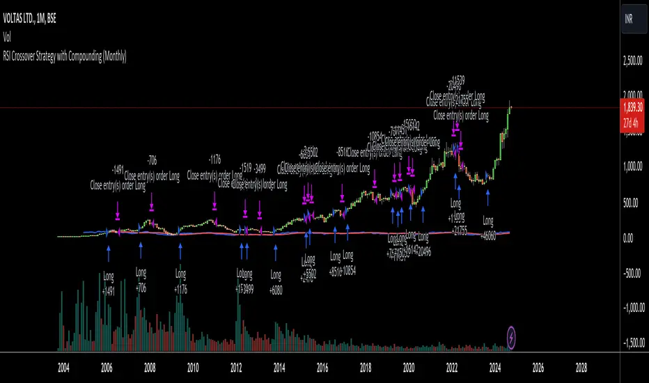
RSI Crossover Strategy with Compounding (Monthly)Explanation of the Code:
Initial Setup:
The strategy initializes with a capital of 100,000.
Variables track the capital and the amount invested in the current trade.
RSI Calculation:
The RSI and its SMA are calculated on the monthly timeframe using request.security().
Entry and Exit Conditions:
Entry: A long position is initiated when the RSI is above its SMA and there’s no existing position. The quantity is based on available capital.
Exit: The position is closed when the RSI falls below its SMA. The capital is updated based on the net profit from the trade.
Capital Management:
After closing a trade, the capital is updated with the net profit plus the initial investment.
Plotting:
The RSI and its SMA are plotted for visualization on the chart.
A label displays the current capital.
Notes:
Test the strategy on different instruments and historical data to see how it performs.
Adjust parameters as needed for your specific trading preferences.
This script is a basic framework, and you might want to enhance it with risk management, stop-loss, or take-profit features as per your trading strategy.
Feel free to modify it further based on your needs!
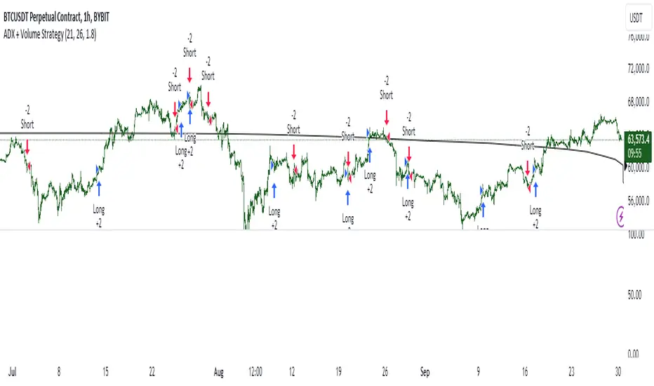
ADX + Volume Strategy### Strategy Description: ADX and Volume-Based Trading Strategy
This strategy is designed to identify strong market trends using the **Average Directional Index (ADX)** and confirm trading signals with **Volume**. The idea behind the strategy is to enter trades only when the market shows a strong trend (as indicated by ADX) and when the price movement is supported by high trading volume. This combination helps filter out weaker signals and provides more reliable entries into positions.
### Key Indicators:
1. **ADX (Average Directional Index)**:
- **Purpose**: ADX is a technical indicator that measures the strength of a trend, regardless of its direction (up or down).
- **Usage**: The strategy uses ADX to determine whether the market is trending strongly. If ADX is above a certain threshold (default is 25), it indicates that a strong trend is present.
- **Directional Indicators**:
- **DI+ (Directional Indicator Plus)**: Indicates the strength of the upward price movement.
- **DI- (Directional Indicator Minus)**: Indicates the strength of the downward price movement.
- ADX does not indicate the direction of the trend but confirms that a trend exists. DI+ and DI- are used to determine the direction.
2. **Volume**:
- **Purpose**: Volume is a key indicator for confirming the strength of a price movement. High volume suggests that a large number of market participants are supporting the movement, making it more likely to continue.
- **Usage**: The strategy compares the current volume to the 20-period moving average of the volume. The trade signal is confirmed if the current volume is greater than the average volume by a specified **Volume Multiplier** (default multiplier is 1.5). This ensures that the trade is supported by strong market participation.
### Strategy Logic:
#### **Entry Conditions:**
1. **Long Position** (Buy):
- **ADX** is above the threshold (default is 25), indicating a strong trend.
- **DI+ > DI-**, signaling that the market is trending upward.
- The **current volume** is greater than the 20-period average volume multiplied by the **Volume Multiplier** (e.g., 1.5), indicating that the upward price movement is backed by sufficient market activity.
2. **Short Position** (Sell):
- **ADX** is above the threshold (default is 25), indicating a strong trend.
- **DI- > DI+**, signaling that the market is trending downward.
- The **current volume** is greater than the 20-period average volume multiplied by the **Volume Multiplier** (e.g., 1.5), indicating that the downward price movement is backed by strong selling activity.
#### **Exit Conditions**:
- Positions are closed when the opposite signal appears:
- **For long positions**: Close when the short conditions are met (ADX still above the threshold, DI- > DI+, and the volume condition holds).
- **For short positions**: Close when the long conditions are met (ADX still above the threshold, DI+ > DI-, and the volume condition holds).
### Parameters:
- **ADX Period**: The period used to calculate ADX (default is 14). This controls how sensitive the ADX is to price movements.
- **ADX Threshold**: The minimum ADX value required for the strategy to consider the market trend as strong (default is 25). Higher values focus on stronger trends.
- **Volume Multiplier**: This parameter adjusts how much higher the current volume needs to be compared to the 20-period moving average for the signal to be valid. A value of 1.5 means the current volume must be 50% higher than the average volume.
### Example Trade Flow:
1. **Long Trade Example**:
- ADX > 25, confirming a strong trend.
- DI+ > DI-, confirming that the trend direction is upward.
- The current volume is 50% higher than the 20-period average volume (multiplied by 1.5).
- **Action**: Enter a long position.
2. **Short Trade Example**:
- ADX > 25, confirming a strong trend.
- DI- > DI+, confirming that the trend direction is downward.
- The current volume is 50% higher than the 20-period average volume.
- **Action**: Enter a short position.
### Strengths of the Strategy:
- **Trend Filtering**: The strategy ensures that trades are only taken when the market is trending strongly (confirmed by ADX) and that the price movement is supported by high volume, reducing the likelihood of false signals.
- **Volume Confirmation**: Using volume as confirmation provides an additional layer of reliability, as volume spikes often accompany sustained price moves.
- **Dual Signal Confirmation**: Both trend strength (ADX) and volume conditions must be met for a trade, making the strategy more robust.
### Weaknesses of the Strategy:
- **Limited Effectiveness in Range-Bound Markets**: Since the strategy relies on strong trends, it may underperform in sideways or non-trending markets where ADX stays below the threshold.
- **Lagging Nature of ADX**: ADX is a lagging indicator, which means that it may confirm the trend after it has already begun, potentially leading to late entries.
- **Volume Requirement**: In low-volume markets, the volume multiplier condition may not be met often, leading to fewer trade opportunities.
### Customization:
- **Adjust the ADX Threshold**: You can raise the threshold if you want to focus only on very strong trends, or lower it to capture moderate trends.
- **Adjust the Volume Multiplier**: You can change the multiplier to be more or less strict. A higher multiplier (e.g., 2.0) will require a stronger volume spike to confirm the signal, while a lower multiplier (e.g., 1.2) will allow more trades with weaker volume confirmation.
### Summary:
This ADX and Volume strategy is ideal for traders who want to follow strong trends while ensuring that the trend is supported by high trading volume. By combining a trend strength filter (ADX) and volume confirmation, the strategy aims to increase the probability of entering profitable trades while reducing the number of false signals. However, it may underperform in range-bound markets or in markets with low volume.
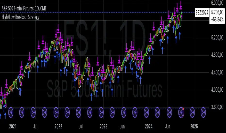
High/Low Breakout Statistical Analysis StrategyThis Pine Script strategy is designed to assist in the statistical analysis of breakout systems on a monthly, weekly, or daily timeframe. It allows the user to select whether to open a long or short position when the price breaks above or below the respective high or low for the chosen timeframe. The user can also define the holding period for each position in terms of bars.
Core Functionality:
Breakout Logic:
The strategy triggers trades based on price crossing over (for long positions) or crossing under (for short positions) the high or low of the selected period (daily, weekly, or monthly).
Timeframe Selection:
A dropdown menu enables the user to switch between the desired timeframe (monthly, weekly, or daily).
Trade Direction:
Another dropdown allows the user to select the type of trade (long or short) depending on whether the breakout occurs at the high or low of the timeframe.
Holding Period:
Once a trade is opened, it is automatically closed after a user-defined number of bars, making it useful for analyzing how breakout signals perform over short-term periods.
This strategy is intended exclusively for research and statistical purposes rather than real-time trading, helping users to assess the behavior of breakouts over different timeframes.
Relevance of Breakout Systems:
Breakout trading systems, where trades are executed when the price moves beyond a significant price level such as the high or low of a given period, have been extensively studied in financial literature for their potential predictive power.
Momentum and Trend Following:
Breakout strategies are a form of momentum-based trading, exploiting the tendency of prices to continue moving in the direction of a strong initial movement after breaching a critical support or resistance level. According to academic research, momentum strategies, including breakouts, can produce returns above average market returns when applied consistently. For example, Jegadeesh and Titman (1993) demonstrated that stocks that performed well in the past 3-12 months continued to outperform in the subsequent months, suggesting that price continuation patterns, like breakouts, hold value .
Market Efficiency Hypothesis:
While the Efficient Market Hypothesis (EMH) posits that markets are generally efficient, and it is difficult to outperform the market through technical strategies, some studies show that in less liquid markets or during specific times of market stress, breakout systems can capitalize on temporary inefficiencies. Taylor (2005) and other researchers have found instances where breakout systems can outperform the market under certain conditions.
Volatility and Breakouts:
Breakouts are often linked to periods of increased volatility, which can generate trading opportunities. Coval and Shumway (2001) found that periods of heightened volatility can make breakouts more significant, increasing the likelihood that price trends will follow the breakout direction. This correlation between volatility and breakout reliability makes it essential to study breakouts across different timeframes to assess their potential profitability .
In summary, this breakout strategy offers an empirical way to study price behavior around key support and resistance levels. It is useful for researchers and traders aiming to statistically evaluate the effectiveness and consistency of breakout signals across different timeframes, contributing to broader research on momentum and market behavior.
References:
Jegadeesh, N., & Titman, S. (1993). Returns to Buying Winners and Selling Losers: Implications for Stock Market Efficiency. Journal of Finance, 48(1), 65-91.
Fama, E. F., & French, K. R. (1996). Multifactor Explanations of Asset Pricing Anomalies. Journal of Finance, 51(1), 55-84.
Taylor, S. J. (2005). Asset Price Dynamics, Volatility, and Prediction. Princeton University Press.
Coval, J. D., & Shumway, T. (2001). Expected Option Returns. Journal of Finance, 56(3), 983-1009.
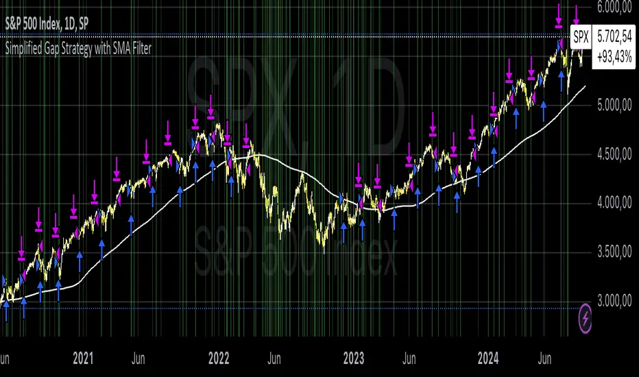
Simplified Gap Strategy with SMA FilterThe Simplified Gap Strategy leverages price gaps as a trading signal, focusing on their significance in market behavior. Gaps occur when the opening price of a security differs significantly from the previous closing price, often signaling potential continuation or reversal patterns.
Key Features:
Gap Threshold:
This strategy requires a minimum percentage gap (defined by the user) to qualify for trading signals.
Directional Trading:
Users can select from various gap types, including "Long Up Gap" and "Short Down Gap," allowing for tailored trading approaches.
SMA Filter:
An optional Simple Moving Average (SMA) filter helps refine trade entries based on trend direction, increasing the probability of successful trades.
Hold Duration:
Positions can be held for a user-defined duration, providing flexibility in trade management.
Statistical Significance of Gaps:
Research has shown that gaps can provide insights into future price movements. According to studies such as those by Hutton and Jiang (2008), price gaps are often followed by momentum in the direction of the gap, indicating that they can serve as reliable indicators for traders. The "Gap Theory" suggests that gaps are filled approximately 90% of the time, emphasizing their relevance in market dynamics (Nikkinen, Sahlström, & Kinnunen, 2006).
Important Note:
This strategy is designed solely for statistical analysis and should not be construed as financial advice. Users are encouraged to conduct their own research and analysis before applying this strategy in live trading scenarios.
By understanding the underlying mechanisms of price gaps and their statistical significance, traders can enhance their decision-making processes and potentially improve trading outcomes.
References:
Hutton, A. W., & Jiang, W. (2008). "Price Gaps: A Guide to Trading Gaps."
Nikkinen, J., Sahlström, P., & Kinnunen, J. (2006). "The Gaps in Financial Markets: An Empirical Study."
This description provides an overview of the strategy while emphasizing its analytical purpose and backing it with relevant academic insights.
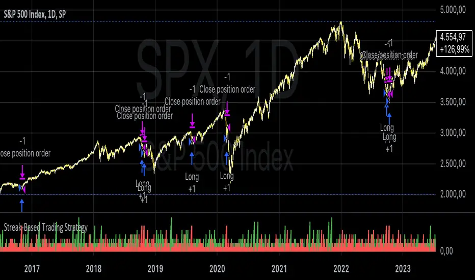
Streak-Based Trading StrategyThe strategy outlined in the provided script is a streak-based trading strategy that focuses on analyzing winning and losing streaks. It’s important to emphasize that this strategy is not intended for actual trading but rather for statistical analysis of streak series.
How the Strategy Works
1. Parameter Definition:
• Trade Direction: Users can choose between “Long” (buy) and “Short” (sell).
• Streak Threshold: Defines how many consecutive wins or losses are needed to trigger a trade.
• Hold Duration: Specifies how many periods the position will be held.
• Doji Threshold: Determines the sensitivity for Doji candles, which indicate market uncertainty.
2. Streak Calculation:
• The script identifies Doji candles and counts winning and losing streaks based on the closing price compared to the previous closing price.
• Streak counting occurs only when no position is currently held.
3. Trade Conditions:
• If the loss streak reaches the defined threshold and the trade direction is “Long,” a buy position is opened.
• If the win streak is met and the trade direction is “Short,” a sell position is opened.
• The position is held for the specified duration.
4. Visualization:
• Winning and losing streaks are plotted as histograms to facilitate analysis.
Scientific Basis
The concept of analyzing streaks in financial markets is well-documented in behavioral economics and finance. Studies have shown that markets often exhibit momentum and trend-following behavior, meaning the likelihood of consecutive winning or losing periods can be higher than what random statistics would suggest (see, for example, “The Behavior of Stock-Market Prices” by Eugene Fama).
Additionally, empirical research indicates that investors often make decisions based on psychological factors influenced by streaks. This can lead to irrational behavior, as they may focus on past wins or losses (see “Behavioral Finance: Psychology, Decision-Making, and Markets” by R. M. F. F. Thaler).
Overall, this strategy serves as a tool for statistical analysis of streak series, providing deeper insights into market behavior and trends rather than being directly used for trading decisions.
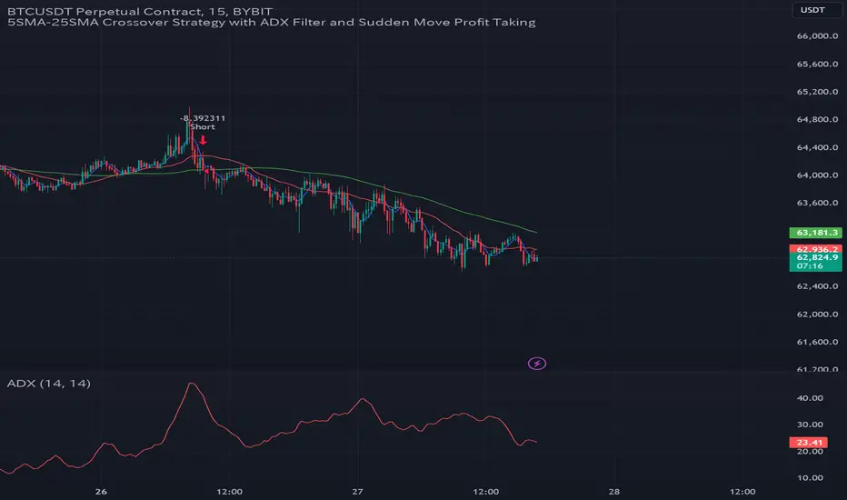
GC Strategy with Trend Filter and Sudden Move Profit TakingBYBIT:BTCUSDT.P 15M
Situation Assessment with Three Moving Averages
The strategy uses the crossover of the 5SMA and 25SMA as entry signals.
Additionally, the 75SMA is used as a filter. Long entries are only allowed when the price is above the 75SMA, and short entries are only allowed when the price is below the 75SMA.
ADX Filter
The Average Directional Index (ADX) is used to check the strength of the trend. Entry signals are only activated when the ADX is above 20. This ensures that trades are only executed when the trend is strong.
Sudden Move Detection
The strategy detects sudden price movements. If a sudden move occurs, the position is closed to lock in profits.
Entry
Long Entry: When the 5SMA crosses above the 25SMA, the price is above the 75SMA, and the ADX is above 20.
Short Entry: When the 5SMA crosses below the 25SMA, the price is below the 75SMA, and the ADX is above 20.
Exit
Positions are closed if a sudden move occurs. Positions are also closed if an opposing entry signal is generated.
This strategy aims to confirm the strength of the trend using moving average crossovers and ADX and to lock in profits based on sudden price movements.
3本の移動平均線による状況判断
5SMAと25SMA のクロスオーバーをエントリーシグナルとして使用します。
さらに、75SMAをフィルターとして使用し、価格が75SMAの上にある場合のみロングエントリーを許可し、75SMAの下にある場合のみショートエントリーを許可します。
ADXフィルター
ADX(平均方向性指数)を使ってトレンドの強さを確認します。
ADXが20より大きい場合のみ、エントリーシグナルを有効にします。これにより、トレンドが強い時にのみ取引を行うことができます。
急激な変動検知
価格の急激な変動を検出します。
急激な変動があった場合には、ポジションをクローズして利益を確定します。
エントリー
ロングエントリー
5SMAが25SMAを上にクロスし、価格が75SMAの上にあり、ADXが20を超えているとき。
ショートエントリー
5SMAが25SMAを下にクロスし、価格が75SMAの下にあり、ADXが20を超えているとき。
エグジット
急激な変動があった場合、ポジションをクローズします。
反対のエントリーシグナルが発生した場合にも、ポジションをクローズします。
このストラテジーは、移動平均のクロスオーバーとADXを使ってトレンドの強さを確認し、急激な変動に基づいて利益を確定することを目的としています。
Fibonacci-Only StrategyFibonacci-Only Strategy
This script is a custom trading strategy designed for traders who leverage Fibonacci retracement levels to identify potential trade entries and exits. The strategy is versatile, allowing users to trade across multiple timeframes, with built-in options for dynamic stop loss, trailing stops, and take profit levels.
Key Features:
Custom Fibonacci Levels:
This strategy calculates three specific Fibonacci retracement levels: 19%, 82.56%, and the reverse 19% level. These levels are used to identify potential areas of support and resistance where price reversals or breaks might occur.
The Fibonacci levels are calculated based on the highest and lowest prices within a 100-bar period, making them dynamic and responsive to recent market conditions.
Dynamic Entry Conditions:
Touch Entry: The script enters long or short positions when the price touches specific Fibonacci levels and confirms the move with a bullish (for long) or bearish (for short) candle.
Break Entry (Optional): If the "Use Break Strategy" option is enabled, the script can also enter positions when the price breaks through Fibonacci levels, providing more aggressive entry opportunities.
Stop Loss Management:
The script offers flexible stop loss settings. Users can choose between a fixed percentage stop loss or an ATR-based stop loss, which adjusts based on market volatility.
The ATR (Average True Range) stop loss is multiplied by a user-defined factor, allowing for tailored risk management based on market conditions.
Trailing Stop Mechanism:
The script includes an optional trailing stop feature, which adjusts the stop loss level as the market moves in favor of the trade. This helps lock in profits while allowing the trade to run if the trend continues.
The trailing stop is calculated as a percentage of the difference between the entry price and the current market price.
Multiple Take Profit Levels:
The strategy calculates seven take profit levels, each at incremental percentages above (for long trades) or below (for short trades) the entry price. This allows for gradual profit-taking as the market moves in the trade's favor.
Each take profit level can be customized in terms of the percentage of the position to be closed, providing precise control over exit strategies.
Strategy Backtesting and Results:
Realistic Backtesting:
The script has been backtested with realistic account sizes, commission rates, and slippage settings to ensure that the results are applicable to actual trading scenarios.
The backtesting covers various timeframes and markets to ensure the strategy's robustness across different trading environments.
Default Settings:
The script is published with default settings that have been optimized for general use. These settings include a 15-minute timeframe, a 1.0% stop loss, a 2.0 ATR multiplier for stop loss, and a 1.5% trailing stop.
Users can adjust these settings to better fit their specific trading style or the market they are trading.
How It Works:
Long Entry Conditions:
The strategy enters a long position when the price touches the 19% Fibonacci level (from high to low) or the reverse 19% level (from low to high) and confirms the move with a bullish candle.
If the "Use Break Strategy" option is enabled, the script will also enter a long position when the price breaks below the 19% Fibonacci level and then moves back up, confirming the break with a bullish candle.
Short Entry Conditions:
The strategy enters a short position when the price touches the 82.56% Fibonacci level and confirms the move with a bearish candle.
If the "Use Break Strategy" option is enabled, the script will also enter a short position when the price breaks above the 82.56% Fibonacci level and then moves back down, confirming the break with a bearish candle.
Stop Loss and Take Profit Logic:
The stop loss for each trade is calculated based on the selected method (fixed percentage or ATR-based). The strategy then manages the trade by either trailing the stop or taking profit at predefined levels.
The take profit levels are set at increments of 0.5% above or below the entry price, depending on whether the position is long or short. The script gradually exits the trade as these levels are hit, securing profits while minimizing risk.
Usage:
For Fibonacci Traders:
This script is ideal for traders who rely on Fibonacci retracement levels to find potential trade entries and exits. The script automates the process, allowing traders to focus on market analysis and decision-making.
For Trend and Swing Traders:
The strategy's flexibility in handling both touch and break entries makes it suitable for trend-following and swing trading strategies. The multiple take profit levels allow traders to capture profits in trending markets while managing risk.
Important Notes:
Originality: This script uniquely combines Fibonacci retracement levels with dynamic stop loss management and multiple take profit levels. It is not just a combination of existing indicators but a thoughtful integration designed to enhance trading performance.
Disclaimer: Trading involves risk, and it is crucial to test this script in a demo account or through backtesting before applying it to live trading. Users should ensure that the settings align with their individual risk tolerance and trading strategy.

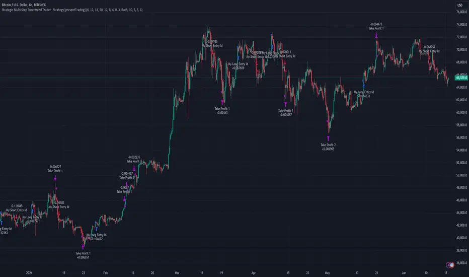
Strategic Multi-Step Supertrend - Strategy [presentTrading]The code is mainly developed for me to stimulate the multi-step taking profit function for strategies. The result shows the drawdown can be reduced but at the same time reduced the profit as well. It can be a heuristic for futures leverage traders.
█ Introduction and How it is Different
The "Strategic Multi-Step Supertrend" is a trading strategy designed to leverage the power of multiple steps to optimize trade entries and exits across the Supertrend indicator. Unlike traditional strategies that rely on single entry and exit points, this strategy employs a multi-step approach to take profit, allowing traders to lock in gains incrementally. Additionally, the strategy is adaptable to both long and short trades, providing a comprehensive solution for dynamic market conditions.
This template strategy lies in its dual Supertrend calculation, which enhances the accuracy of trend detection and provides more reliable signals for trade entries and exits. This approach minimizes false signals and increases the overall profitability of trades by ensuring that positions are entered and exited at optimal points.
BTC 6h L/S Performance
█ Strategy, How It Works: Detailed Explanation
The "Strategic Multi-Step Supertrend Trader" strategy utilizes two Supertrend indicators calculated with different parameters to determine the direction and strength of the market trend. This dual approach increases the robustness of the signals, reducing the likelihood of entering trades based on false signals. Here is a detailed breakdown of how the strategy operates:
🔶 Supertrend Indicator Calculation
The Supertrend indicator is a trend-following overlay on the price chart, typically used to identify the direction of the trend. It is calculated using the Average True Range (ATR) to ensure that the indicator adapts to market volatility. The formula for the Supertrend indicator is:
Upper Band = (High + Low) / 2 + (Factor * ATR)
Lower Band = (High + Low) / 2 - (Factor * ATR)
Where:
- High and Low are the highest and lowest prices of the period.
- Factor is a user-defined multiplier.
- ATR is the Average True Range over a specified period.
The Supertrend changes its direction based on the closing price in relation to these bands.
🔶 Entry-Exit Conditions
The strategy enters long positions when both Supertrend indicators signal an uptrend, and short positions when both indicate a downtrend. Specifically:
- Long Condition: Supertrend1 < 0 and Supertrend2 < 0
- Short Condition: Supertrend1 > 0 and Supertrend2 > 0
- Long Exit Condition: Supertrend1 > 0 and Supertrend2 > 0
- Short Exit Condition: Supertrend1 < 0 and Supertrend2 < 0
🔶 Multi-Step Take Profit Mechanism
The strategy features a multi-step take profit mechanism, which allows traders to lock in profits incrementally. This is achieved through four user-configurable take profit levels. For each level, the strategy specifies a percentage increase (for long trades) or decrease (for short trades) in the entry price at which a portion of the position is exited:
- Step 1: Exit a portion of the trade at Entry Price * (1 + Take Profit Percent1 / 100)
- Step 2: Exit a portion of the trade at Entry Price * (1 + Take Profit Percent2 / 100)
- Step 3: Exit a portion of the trade at Entry Price * (1 + Take Profit Percent3 / 100)
- Step 4: Exit a portion of the trade at Entry Price * (1 + Take Profit Percent4 / 100)
This staggered exit strategy helps in locking profits at multiple levels, thereby reducing risk and increasing the likelihood of capturing the maximum possible profit from a trend.
BTC Local
█ Trade Direction
The strategy is highly flexible, allowing users to specify the trade direction. There are three options available:
- Long Only: The strategy will only enter long trades.
- Short Only: The strategy will only enter short trades.
- Both: The strategy will enter both long and short trades based on the Supertrend signals.
This flexibility allows traders to adapt the strategy to various market conditions and their own trading preferences.
█ Usage
1. Add the strategy to your trading platform and apply it to the desired chart.
2. Configure the take profit settings under the "Take Profit Settings" group.
3. Set the trade direction under the "Trade Direction" group.
4. Adjust the Supertrend settings in the "Supertrend Settings" group to fine-tune the indicator calculations.
5. Monitor the chart for entry and exit signals as indicated by the strategy.
█ Default Settings
- Use Take Profit: True
- Take Profit Percentages: Step 1 - 6%, Step 2 - 12%, Step 3 - 18%, Step 4 - 50%
- Take Profit Amounts: Step 1 - 12%, Step 2 - 8%, Step 3 - 4%, Step 4 - 0%
- Number of Take Profit Steps: 3
- Trade Direction: Both
- Supertrend Settings: ATR Length 1 - 10, Factor 1 - 3.0, ATR Length 2 - 11, Factor 2 - 4.0
These settings provide a balanced starting point, which can be customized further based on individual trading preferences and market conditions.
Adaptive RSI StrategyThe Adaptive RSI Strategy is designed to give you an edge by adapting to changing market conditions more effectively than the traditional RSI. By adjusting dynamically to recent price movements, this strategy aims to provide more timely and accurate trade signals.
How Does It Work?
You can set the number of periods for the RSI calculation. The default is 14, but feel free to experiment with different lengths to suit your trading style.
Choose the price data to base the RSI on, typically the closing price.
Decide if you want the strategy to visually highlight upward and downward movements of the Adaptive RSI (ARSI) on the chart. This can help you quickly spot trends.
Adaptive Calculation:
Alpha: The strategy uses an adaptive factor called alpha, which changes based on recent RSI values. This makes the RSI more sensitive to recent market conditions.
Adaptive RSI (ARSI): This is the core of our strategy. It calculates the ARSI using the adaptive alpha, making it more responsive to price changes compared to the traditional RSI.
Trade Signals:
Long Entry (Buy Signal): The strategy triggers a buy signal when the ARSI value crosses above its previous value. This indicates a potential upward trend, suggesting it's a good time to enter a long position.
Short Entry (Sell Signal): Conversely, a sell signal is triggered when the ARSI value crosses below its previous value, indicating a potential downward trend and suggesting it's a good time to enter a short position.
Visual Representation:
If you enable the highlight movements feature, the ARSI line on the chart will change color: green for upward movements and red for downward movements. This makes it easier to see potential trade opportunities at a glance.
Why Use the Adaptive RSI Strategy?
Responsiveness: The adaptive nature of this strategy means it's more sensitive to market changes, helping you react quicker to new trends.
Customization: You can tailor the length of the RSI period and decide whether to highlight movements, allowing you to adapt the strategy to your specific needs and preferences.
Visual Clarity: Highlighting the ARSI movements on the chart makes it easier to spot trends and potential entry points, giving you a clearer picture of the market.
Trailing Take Profit - Close Based📝 Description
This script demonstrates a new approach to the trailing take profit.
Trailing Take Profit is a price-following technique. When used, instead of setting a limit order for the take profit target exiting from your position at the specified price, a stop order is conditionally set when the take profit target is reached. Then, the stop price (a.k.a trailing price), is placed below the take profit target at a distance defined by the user percentagewise. On regular time intervals, the stop price gets updated by following the "Trail Barrier" price (high by default) upwards. When the current price hits the stop price you exit the trade. Check the chart for more details.
This script demonstrates how to implement the close-based Trailing Take Profit logic for long positions, but it can also be applied for short positions if the logic is "reversed".
📢 NOTE
To generate some entries and showcase the "Trailing Take Profit" technique, this script uses the crossing of two moving averages. Please keep in mind that you should not relate the Backtesting results you see in the "Strategy Tester" tab with the success of the technique itself.
This is not a complete strategy per se, and the backtest results are affected by many parameters that are outside of the scope of this publication. If you choose to use this new approach of the "Trailing Take Profit" in your logic you have to make sure that you are backtesting the whole strategy.
⚔️ Comparison
In contrast to my older "Trailing Take Profit" publication where the trailing take profit implementation was tick-based, this new approach is close-based, meaning that the update of the stop price occurs at the bar close instead of every tick.
While comparing the real-time results of the two implementations is like comparing apples to oranges, because they have different dynamic behavior, the new approach offers better consistency between the backtesting results and the real-time results.
By updating the stop price on every bar close, you do not rely on the backtester assumptions anymore (check the Reasoning section below for more info).
The new approach resembles the conditional "Trailing Exit" technique, where the condition is true when the current price crosses over the take profit target. Then, the stop order is placed at the trailing price and it gets updated on every bar close to "follow" the barrier price (high). On the other hand, the older tick-based approach had more "tight" dynamics since the trailing price gets updated on every tick leaving less room for price fluctuations by making it more probable to reach the trailing price.
🤔 Reasoning
This new close-based approach addresses several practical issues the older tick-based approach had. Those issues arise mainly from the technicalities of the TV Backtester. More specifically, due to the assumptions the Broker Emulator makes for the price action of the history bars, the backtesting results in the TV Backtester are exaggerated, and depending on the timeframe, the backtesting results look way better than they are in reality.
The effect above, and the inability to reason about the performance of a strategy separated people into two groups. Those who never use this feature, because they couldn't know for sure the actual effect it might have in their strategy, (even if it turned out to be more profitable) and those who abused this type of "repainting" behavior to show off, and hijack some boosts from the community by boasting about the "fake" results of their strategies.
Even if there are ways to evaluate the effectiveness of the tick-based approach that is applied in an existing strategy (this is out of the topic of this publication), it requires extra effort to do the analysis. Using this closed-based approach we can have more predictable results, without surprises.
⚠️ Caveats
Since this approach updates the trailing price on bar close, you must wait for at least one bar to close after the price crosses over the take profit target.
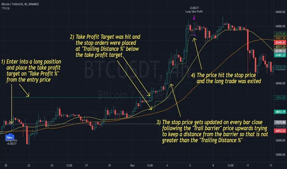
Bitcoin 5A Strategy@LilibtcIn our long-term strategy, we have deeply explored the key factors influencing the price of Bitcoin. By precisely calculating the correlation between these factors and the price of Bitcoin, we found that they are closely linked to the value of Bitcoin. To more effectively predict the fair price of Bitcoin, we have built a predictive model and adjusted our investment strategy accordingly based on this model. In practice, the prediction results of this model correspond quite high with actual values, fully demonstrating its reliability in predicting price fluctuations.
When the future is uncertain and the outlook is unclear, people often choose to hold back and avoid risks, or even abandon their original plans. However, the prediction of Bitcoin is full of challenges, but we have taken the first step in exploring.
Table of contents:
Usage Guide
Step 1: Identify the factors that have the greatest impact on Bitcoin price
Step 2: Build a Bitcoin price prediction model
Step 3: Find indicators for warning of bear market bottoms and bull market tops
Step 4: Predict Bitcoin Price in 2025
Step 5: Develop a Bitcoin 5A strategy
Step 6: Verify the performance of the Bitcoin 5A strategy
Usage Restrictions
🦮Usage Guide:
1. On the main interface, modify the code, find the BTCUSD trading pair, and select the BITSTAMP exchange for trading.
2. Set the time period to the daily chart.
3. Select a logarithmic chart in the chart type to better identify price trends.
4. In the strategy settings, adjust the options according to personal needs, including language, display indicators, display strategies, display performance, display optimizations, sell alerts, buy prompts, opening days, backtesting start year, backtesting start month, and backtesting start date.
🏃Step 1: Identify the factors that have the greatest impact on Bitcoin price
📖Correlation Coefficient: A mathematical concept for measuring influence
In order to predict the price trend of Bitcoin, we need to delve into the factors that have the greatest impact on its price. These factors or variables can be expressed in mathematical or statistical correlation coefficients. The correlation coefficient is an indicator of the degree of association between two variables, ranging from -1 to 1. A value of 1 indicates a perfect positive correlation, while a value of -1 indicates a perfect negative correlation.
For example, if the price of corn rises, the price of live pigs usually rises accordingly, because corn is the main feed source for pig breeding. In this case, the correlation coefficient between corn and live pig prices is approximately 0.3. This means that corn is a factor affecting the price of live pigs. On the other hand, if a shooter's performance improves while another shooter's performance deteriorates due to increased psychological pressure, we can say that the former is a factor affecting the latter's performance.
Therefore, in order to identify the factors that have the greatest impact on the price of Bitcoin, we need to find the factors with the highest correlation coefficients with the price of Bitcoin. If, through the analysis of the correlation between the price of Bitcoin and the data on the chain, we find that a certain data factor on the chain has the highest correlation coefficient with the price of Bitcoin, then this data factor on the chain can be identified as the factor that has the greatest impact on the price of Bitcoin. Through calculation, we found that the 🔵number of Bitcoin blocks is one of the factors that has the greatest impact on the price of Bitcoin. From historical data, it can be clearly seen that the growth rate of the 🔵number of Bitcoin blocks is basically consistent with the movement direction of the price of Bitcoin. By analyzing the past ten years of data, we obtained a daily correlation coefficient of 0.93 between the number of Bitcoin blocks and the price of Bitcoin.
🏃Step 2: Build a Bitcoin price prediction model
📖Predictive Model: What formula is used to predict the price of Bitcoin?
Among various prediction models, the linear function is the preferred model due to its high accuracy. Take the standard weight as an example, its linear function graph is a straight line, which is why we choose the linear function model. However, the growth rate of the price of Bitcoin and the number of blocks is extremely fast, which does not conform to the characteristics of the linear function. Therefore, in order to make them more in line with the characteristics of the linear function, we first take the logarithm of both. By observing the logarithmic graph of the price of Bitcoin and the number of blocks, we can find that after the logarithm transformation, the two are more in line with the characteristics of the linear function. Based on this feature, we choose the linear regression model to establish the prediction model.
From the graph below, we can see that the actual red and green K-line fluctuates around the predicted blue and 🟢green line. These predicted values are based on fundamental factors of Bitcoin, which support its value and reflect its reasonable value. This picture is consistent with the theory proposed by Marx in "Das Kapital" that "prices fluctuate around values."
The predicted logarithm of the market cap of Bitcoin is calculated through the model. The specific calculation formula of the Bitcoin price prediction value is as follows:
btc_predicted_marketcap = math.exp(btc_predicted_marketcap_log)
btc_predicted_price = btc_predicted_marketcap / btc_supply
🏃Step 3: Find indicators for early warning of bear market bottoms and bull market tops
📖Warning Indicator: How to Determine Whether the Bitcoin Price has Reached the Bear Market Bottom or the Bull Market Top?
By observing the Bitcoin price logarithmic prediction chart mentioned above, we notice that the actual price often falls below the predicted value at the bottom of a bear market; during the peak of a bull market, the actual price exceeds the predicted price. This pattern indicates that the deviation between the actual price and the predicted price can serve as an early warning signal. When the 🔴 Bitcoin price deviation is very low, as shown by the chart with 🟩green background, it usually means that we are at the bottom of the bear market; Conversely, when the 🔴 Bitcoin price deviation is very high, the chart with a 🟥red background indicates that we are at the peak of the bull market.
This pattern has been validated through six bull and bear markets, and the deviation value indeed serves as an early warning signal, which can be used as an important reference for us to judge market trends.
🏃Step 4:Predict Bitcoin Price in 2025
📖Price Upper Limit
According to the data calculated on February 25, 2024, the 🟠upper limit of the Bitcoin price is $194,287, which is the price ceiling of this bull market. The peak of the last bull market was on November 9, 2021, at $68,664. The bull-bear market cycle is 4 years, so the highest point of this bull market is expected in 2025. That is where you should sell the Bitcoin. and the upper limit of the Bitcoin price will exceed $190,000. The closing price of Bitcoin on February 25, 2024, was $51,729, with an expected increase of 2.7 times.
🏃Step 5: Bitcoin 5A Strategy Formulation
📖Strategy: When to buy or sell, and how many to choose?
We introduce the Bitcoin 5A strategy. This strategy requires us to generate trading signals based on the critical values of the warning indicators, simulate the trades, and collect performance data for evaluation. In the Bitcoin 5A strategy, there are three key parameters: buying warning indicator, batch trading days, and selling warning indicator. Batch trading days are set to ensure that we can make purchases in batches after the trading signal is sent, thus buying at a lower price, selling at a higher price, and reducing the trading impact cost.
In order to find the optimal warning indicator critical value and batch trading days, we need to adjust these parameters repeatedly and perform backtesting. Backtesting is a method established by observing historical data, which can help us better understand market trends and trading opportunities.
Specifically, we can find the key trading points by watching the Bitcoin price log and the Bitcoin price deviation chart. For example, on August 25, 2015, the 🔴 Bitcoin price deviation was at its lowest value of -1.11; on December 17, 2017, the 🔴 Bitcoin price deviation was at its highest value at the time, 1.69; on March 16, 2020, the 🔴 Bitcoin price deviation was at its lowest value at the time, -0.91; on March 13, 2021, the 🔴 Bitcoin price deviation was at its highest value at the time, 1.1; on December 31, 2022, the 🔴 Bitcoin price deviation was at its lowest value at the time, -1.
To ensure that all five key trading points generate trading signals, we set the warning indicator Bitcoin price deviation to the larger of the three lowest values, -0.9, and the smallest of the two highest values, 1. Then, we buy when the warning indicator Bitcoin price deviation is below -0.9, and sell when it is above 1.
In addition, we set the batch trading days as 25 days to implement a strategy that averages purchases and sales. Within these 25 days, we will invest all funds into the market evenly, buying once a day. At the same time, we also sell positions at the same pace, selling once a day.
📖Adjusting the threshold: a key step to optimizing trading strategy
Adjusting the threshold is an indispensable step for better performance. Here are some suggestions for adjusting the batch trading days and critical values of warning indicators:
• Batch trading days: Try different days like 25 to see how it affects overall performance.
• Buy and sell critical values for warning indicators: iteratively fine-tune the buy threshold value of -0.9 and the sell threshold value of 1 exhaustively to find the best combination of threshold values.
Through such careful adjustments, we may find an optimized approach with a lower maximum drawdown rate (e.g., 11%) and a higher cumulative return rate for closed trades (e.g., 474 times). The chart below is a backtest optimization chart for the Bitcoin 5A strategy, providing an intuitive display of strategy adjustments and optimizations.
In this way, we can better grasp market trends and trading opportunities, thereby achieving a more robust and efficient trading strategy.
🏃Step 6: Validating the performance of the Bitcoin 5A Strategy
📖Model interpretability validation: How to explain the Bitcoin price model?
The interpretability of the model is represented by the coefficient of determination R squared, which reflects the degree of match between the predicted value and the actual value. I divided all the historical data from August 18, 2015 into two groups, and used the data from August 18, 2011 to August 18, 2015 as training data to generate the model. The calculation result shows that the coefficient of determination R squared during the 2011-2015 training period is as high as 0.81, which shows that the interpretability of this model is quite high. From the Bitcoin price logarithmic prediction chart in the figure below, we can see that the deviation between the predicted value and the actual value is not far, which means that most of the predicted values can explain the actual value well.
The calculation formula for the coefficient of determination R squared is as follows:
residual = btc_close_log - btc_predicted_price_log
residual_square = residual * residual
train_residual_square_sum = math.sum(residual_square, train_days)
train_mse = train_residual_square_sum / train_days
train_r2 = 1 - train_mse / ta.variance(btc_close_log, train_days)
📖Model stability verification: How to affirm the stability of the Bitcoin price model when new data is available?
Model stability is achieved through model verification. I set the last day of the training period to February 2, 2024 as the "verification group" and used it as verification data to verify the stability of the model. This means that after generating the model if there is new data, I will use these new data together with the model for prediction, and then evaluate the interpretability of the model. If the coefficient of determination when using verification data is close to the previous training one and both remain at a high level, then we can consider this model as stability. The coefficient of determination calculated from the validation period data and model prediction results is as high as 0.83, which is close to the previous 0.81, further proving the stability of this model.
📖Performance evaluation: How to accurately evaluate historical backtesting results?
After detailed strategy testing, to ensure the accuracy and reliability of the results, we need to carry out a detailed performance evaluation on the backtest results. The key evaluation indices include:
• Net value curve: As shown in the rose line, it intuitively reflects the growth of the account net value. By observing the net value curve, we can understand the overall performance and profitability of the strategy.
The basic attributes of this strategy are as follows:
Trading range: 2015-8-19 to 2024-2-18, backtest range: 2011-8-18 to 2024-2-18
Initial capital: 1000USD, order size: 1 contract, pyramid: 50 orders, commission rate: 0.2%, slippage: 20 markers.
In the strategy tester overview chart, we also obtained the following key data:
• Net profit rate of closed trades: as high as 474 times, far exceeding the benchmark, as shown in the strategy tester performance summary chart, Bitcoin buys and holds 210 times.
• Number of closed trades and winning percentage: 100 trades were all profitable, showing the stability and reliability of the strategy.
• Drawdown rate & win-loose ratio: The maximum drawdown rate is only 11%, far lower than Bitcoin's 78%. Profit factor, or win-loose ratio, reached 500, further proving the advantage of the strategy.
Through these detailed evaluations, we can see clearly the excellent balance between risk and return of the Bitcoin 5A strategy.
⚠️Usage Restrictions: Strategy Application in Specific Situations
Please note that this strategy is designed specifically for Bitcoin and should not be applied to other assets or markets without authorization. In actual operations, we should make careful decisions according to our risk tolerance and investment goals.

Bitcoin 5A Strategy - Price Upper & Lower Limit@LilibtcIn our long-term strategy, we have deeply explored the key factors influencing the price of Bitcoin. By precisely calculating the correlation between these factors and the price of Bitcoin, we found that they are closely linked to the value of Bitcoin. To more effectively predict the fair price of Bitcoin, we have built a predictive model and adjusted our investment strategy accordingly based on this model. In practice, the prediction results of this model correspond quite high with actual values, fully demonstrating its reliability in predicting price fluctuations.
When the future is uncertain and the outlook is unclear, people often choose to hold back and avoid risks, or even abandon their original plans. However, the prediction of Bitcoin is full of challenges, but we have taken the first step in exploring.
Table of contents:
Usage Guide
Step 1: Identify the factors that have the greatest impact on Bitcoin price
Step 2: Build a Bitcoin price prediction model
Step 3: Find indicators for warning of bear market bottoms and bull market tops
Step 4: Predict Bitcoin Price in 2025
Step 5: Develop a Bitcoin 5A strategy
Step 6: Verify the performance of the Bitcoin 5A strategy
Usage Restrictions
🦮Usage Guide:
1. On the main interface, modify the code, find the BTCUSD trading pair, and select the BITSTAMP exchange for trading.
2. Set the time period to the daily chart.
3. Select a logarithmic chart in the chart type to better identify price trends.
4. In the strategy settings, adjust the options according to personal needs, including language, display indicators, display strategies, display performance, display optimizations, sell alerts, buy prompts, opening days, backtesting start year, backtesting start month, and backtesting start date.
🏃Step 1: Identify the factors that have the greatest impact on Bitcoin price
📖Correlation Coefficient: A mathematical concept for measuring influence
In order to predict the price trend of Bitcoin, we need to delve into the factors that have the greatest impact on its price. These factors or variables can be expressed in mathematical or statistical correlation coefficients. The correlation coefficient is an indicator of the degree of association between two variables, ranging from -1 to 1. A value of 1 indicates a perfect positive correlation, while a value of -1 indicates a perfect negative correlation.
For example, if the price of corn rises, the price of live pigs usually rises accordingly, because corn is the main feed source for pig breeding. In this case, the correlation coefficient between corn and live pig prices is approximately 0.3. This means that corn is a factor affecting the price of live pigs. On the other hand, if a shooter's performance improves while another shooter's performance deteriorates due to increased psychological pressure, we can say that the former is a factor affecting the latter's performance.
Therefore, in order to identify the factors that have the greatest impact on the price of Bitcoin, we need to find the factors with the highest correlation coefficients with the price of Bitcoin. If, through the analysis of the correlation between the price of Bitcoin and the data on the chain, we find that a certain data factor on the chain has the highest correlation coefficient with the price of Bitcoin, then this data factor on the chain can be identified as the factor that has the greatest impact on the price of Bitcoin. Through calculation, we found that the 🔵 number of Bitcoin blocks is one of the factors that has the greatest impact on the price of Bitcoin. From historical data, it can be clearly seen that the growth rate of the 🔵 number of Bitcoin blocks is basically consistent with the movement direction of the price of Bitcoin. By analyzing the past ten years of data, we obtained a daily correlation coefficient of 0.93 between the number of Bitcoin blocks and the price of Bitcoin.
🏃Step 2: Build a Bitcoin price prediction model
📖Predictive Model: What formula is used to predict the price of Bitcoin?
Among various prediction models, the linear function is the preferred model due to its high accuracy. Take the standard weight as an example, its linear function graph is a straight line, which is why we choose the linear function model. However, the growth rate of the price of Bitcoin and the number of blocks is extremely fast, which does not conform to the characteristics of the linear function. Therefore, in order to make them more in line with the characteristics of the linear function, we first take the logarithm of both. By observing the logarithmic graph of the price of Bitcoin and the number of blocks, we can find that after the logarithm transformation, the two are more in line with the characteristics of the linear function. Based on this feature, we choose the linear regression model to establish the prediction model.
From the graph below, we can see that the actual red and green K-line fluctuates around the predicted blue and 🟢green line. These predicted values are based on fundamental factors of Bitcoin, which support its value and reflect its reasonable value. This picture is consistent with the theory proposed by Marx in "Das Kapital" that "prices fluctuate around values."
The predicted logarithm of the market cap of Bitcoin is calculated through the model. The specific calculation formula of the Bitcoin price prediction value is as follows:
btc_predicted_marketcap = math.exp(btc_predicted_marketcap_log)
btc_predicted_price = btc_predicted_marketcap / btc_supply
🏃Step 3: Find indicators for early warning of bear market bottoms and bull market tops
📖Warning Indicator: How to Determine Whether the Bitcoin Price has Reached the Bear Market Bottom or the Bull Market Top?
By observing the Bitcoin price logarithmic prediction chart mentioned above, we notice that the actual price often falls below the predicted value at the bottom of a bear market; during the peak of a bull market, the actual price exceeds the predicted price. This pattern indicates that the deviation between the actual price and the predicted price can serve as an early warning signal. When the 🔴 Bitcoin price deviation is very low, as shown by the chart with 🟩green background, it usually means that we are at the bottom of the bear market; Conversely, when the 🔴 Bitcoin price deviation is very high, the chart with a 🟥red background indicates that we are at the peak of the bull market.
This pattern has been validated through six bull and bear markets, and the deviation value indeed serves as an early warning signal, which can be used as an important reference for us to judge market trends.
🏃Step 4:Predict Bitcoin Price in 2025
📖Price Upper Limit
According to the data calculated on March 10, 2023(If you want to check latest data, please contact with author), the 🟠upper limit of the Bitcoin price is $132,453, which is the price ceiling of this bull market. The peak of the last bull market was on November 9, 2021, at $68,664. The bull-bear market cycle is 4 years, so the highest point of this bull market is expected in 2025, and the 🟠upper limit of the Bitcoin price will exceed $130,000. The closing price of Bitcoin on March 10, 2024, was $68,515, with an expected increase of 90%.
🏃Step 5: Bitcoin 5A Strategy Formulation
📖Strategy: When to buy or sell, and how many to choose?
We introduce the Bitcoin 5A strategy. This strategy requires us to generate trading signals based on the critical values of the warning indicators, simulate the trades, and collect performance data for evaluation. In the Bitcoin 5A strategy, there are three key parameters: buying warning indicator, batch trading days, and selling warning indicator. Batch trading days are set to ensure that we can make purchases in batches after the trading signal is sent, thus buying at a lower price, selling at a higher price, and reducing the trading impact cost.
In order to find the optimal warning indicator critical value and batch trading days, we need to adjust these parameters repeatedly and perform backtesting. Backtesting is a method established by observing historical data, which can help us better understand market trends and trading opportunities.
Specifically, we can find the key trading points by watching the Bitcoin price log and the Bitcoin price deviation chart. For example, on August 25, 2015, the 🔴 Bitcoin price deviation was at its lowest value of -1.11; on December 17, 2017, the 🔴 Bitcoin price deviation was at its highest value at the time, 1.69; on March 16, 2020, the 🔴 Bitcoin price deviation was at its lowest value at the time, -0.91; on March 13, 2021, the 🔴 Bitcoin price deviation was at its highest value at the time, 1.1; on December 31, 2022, the 🔴 Bitcoin price deviation was at its lowest value at the time, -1.
To ensure that all five key trading points generate trading signals, we set the warning indicator Bitcoin price deviation to the larger of the three lowest values, -0.9, and the smallest of the two highest values, 1. Then, we buy when the warning indicator Bitcoin price deviation is below -0.9, and sell when it is above 1.
In addition, we set the batch trading days as 25 days to implement a strategy that averages purchases and sales. Within these 25 days, we will invest all funds into the market evenly, buying once a day. At the same time, we also sell positions at the same pace, selling once a day.
📖Adjusting the threshold: a key step to optimizing trading strategy
Adjusting the threshold is an indispensable step for better performance. Here are some suggestions for adjusting the batch trading days and critical values of warning indicators:
• Batch trading days: Try different days like 25 to see how it affects overall performance.
• Buy and sell critical values for warning indicators: iteratively fine-tune the buy threshold value of -0.9 and the sell threshold value of 1 exhaustively to find the best combination of threshold values.
Through such careful adjustments, we may find an optimized approach with a lower maximum drawdown rate (e.g., 11%) and a higher cumulative return rate for closed trades (e.g., 474 times). The chart below is a backtest optimization chart for the Bitcoin 5A strategy, providing an intuitive display of strategy adjustments and optimizations.
In this way, we can better grasp market trends and trading opportunities, thereby achieving a more robust and efficient trading strategy.
🏃Step 6: Validating the performance of the Bitcoin 5A Strategy
📖Model accuracy validation: How to judge the accuracy of the Bitcoin price model?
The accuracy of the model is represented by the coefficient of determination R square, which reflects the degree of match between the predicted value and the actual value. I divided all the historical data from August 18, 2015 into two groups, and used the data from August 18, 2011 to August 18, 2015 as training data to generate the model. The calculation result shows that the coefficient of determination R squared during the 2011-2015 training period is as high as 0.81, which shows that the accuracy of this model is quite high. From the Bitcoin price logarithmic prediction chart in the figure below, we can see that the deviation between the predicted value and the actual value is not far, which means that most of the predicted values can explain the actual value well.
The calculation formula for the coefficient of determination R square is as follows:
residual = btc_close_log - btc_predicted_price_log
residual_square = residual * residual
train_residual_square_sum = math.sum(residual_square, train_days)
train_mse = train_residual_square_sum / train_days
train_r2 = 1 - train_mse / ta.variance(btc_close_log, train_days)
📖Model reliability verification: How to affirm the reliability of the Bitcoin price model when new data is available?
Model reliability is achieved through model verification. I set the last day of the training period to February 2, 2024 as the "verification group" and used it as verification data to verify the reliability of the model. This means that after generating the model if there is new data, I will use these new data together with the model for prediction, and then evaluate the accuracy of the model. If the coefficient of determination when using verification data is close to the previous training one and both remain at a high level, then we can consider this model as reliable. The coefficient of determination calculated from the validation period data and model prediction results is as high as 0.83, which is close to the previous 0.81, further proving the reliability of this model.
📖Performance evaluation: How to accurately evaluate historical backtesting results?
After detailed strategy testing, to ensure the accuracy and reliability of the results, we need to carry out a detailed performance evaluation on the backtest results. The key evaluation indices include:
• Net value curve: As shown in the rose line, it intuitively reflects the growth of the account net value. By observing the net value curve, we can understand the overall performance and profitability of the strategy.
The basic attributes of this strategy are as follows:
Trading range: 2015-8-19 to 2024-2-18, backtest range: 2011-8-18 to 2024-2-18
Initial capital: 1000USD, order size: 1 contract, pyramid: 50 orders, commission rate: 0.2%, slippage: 20 markers.
In the strategy tester overview chart, we also obtained the following key data:
• Net profit rate of closed trades: as high as 474 times, far exceeding the benchmark, as shown in the strategy tester performance summary chart, Bitcoin buys and holds 210 times.
• Number of closed trades and winning percentage: 100 trades were all profitable, showing the stability and reliability of the strategy.
• Drawdown rate & win-loose ratio: The maximum drawdown rate is only 11%, far lower than Bitcoin's 78%. Profit factor, or win-loose ratio, reached 500, further proving the advantage of the strategy.
Through these detailed evaluations, we can see clearly the excellent balance between risk and return of the Bitcoin 5A strategy.
⚠️Usage Restrictions: Strategy Application in Specific Situations
Please note that this strategy is designed specifically for Bitcoin and should not be applied to other assets or markets without authorization. In actual operations, we should make careful decisions according to our risk tolerance and investment goals.
