EMA 10/55/200 - LONG ONLY MTF (4h with 1D & 1W confirmation)Title: EMA 10/55/200 - Long Only Multi-Timeframe Strategy (4h with 1D & 1W confirmation)
Description:
This strategy is designed for trend-following long entries using a combination of exponential moving averages (EMAs) on the 4-hour chart, confirmed by higher timeframe trends from the daily (1D) and weekly (1W) charts.
🔍 How It Works
🔹 Entry Conditions (4h chart):
EMA 10 crosses above EMA 55 and price is above EMA 55
OR
EMA 55 crosses above EMA 200
OR
EMA 10 crosses above EMA 500
These entries indicate short-term momentum aligning with medium/long-term trend strength.
🔹 Confirmation (multi-timeframe alignment):
Daily (1D): EMA 55 is above EMA 200
Weekly (1W): EMA 55 is above EMA 200
This ensures that we only enter long trades when the higher timeframes support an uptrend, reducing false signals during sideways or bearish markets.
🛑 Exit Conditions
Bearish crossover of EMA 10 below EMA 200 or EMA 500
Stop Loss: 5% below entry price
⚙️ Backtest Settings
Capital allocation per trade: 10% of equity
Commission: 0.1%
Slippage: 2 ticks
These are realistic conditions for crypto, forex, and stocks.
📈 Best Used On
Timeframe: 4h
Instruments: Trending markets like BTC/ETH, FX majors, or growth stocks
Works best in volatile or trending environments
⚠️ Disclaimer
This is a backtest tool and educational resource. Always validate on demo accounts before applying to real capital. Do your own due diligence.
Educational

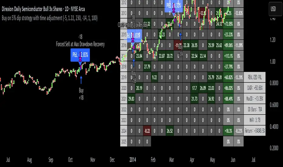
Buy on 5% dip strategy with time adjustment
This script is a strategy called "Buy on 5% Dip Strategy with Time Adjustment 📉💡," which detects a 5% drop in price and triggers a buy signal 🔔. It also automatically closes the position once the set profit target is reached 💰, and it has additional logic to close the position if the loss exceeds 14% after holding for 230 days ⏳.
Strategy Explanation
Buy Condition: A buy signal is triggered when the price drops 5% from the highest price reached 🔻.
Take Profit: The position is closed when the price hits a 1.22x target from the average entry price 📈.
Forced Sell Condition: If the position is held for more than 230 days and the loss exceeds 14%, the position is automatically closed 🚫.
Leverage & Capital Allocation: Leverage is adjustable ⚖️, and you can set the percentage of capital allocated to each trade 💸.
Time Limits: The strategy allows you to set a start and end time ⏰ for trading, making the strategy active only within that specific period.
Code Credits and References
Credits: This script utilizes ideas and code from @QuantNomad and jangdokang for the profit table and algorithm concepts 🔧.
Sources:
Monthly Performance Table Script by QuantNomad:
ZenAndTheArtOfTrading's Script:
Strategy Performance
This strategy provides risk management through take profit and forced sell conditions and includes a performance table 📊 to track monthly and yearly results. You can compare backtest results with real-time performance to evaluate the strategy's effectiveness.
The performance numbers shown in the backtest reflect what would have happened if you had used this strategy since the launch date of the SOXL (the Direxion Daily Semiconductor Bull 3x Shares ETF) 📅. These results are not hypothetical but based on actual performance from the day of the ETF’s launch 📈.
Caution ⚠️
No Guarantee of Future Results: The results are based on historical performance from the launch of the SOXL ETF, but past performance does not guarantee future results. It’s important to approach with caution when applying it to live trading 🔍.
Risk Management: Leverage and capital allocation settings are crucial for managing risk ⚠️. Make sure to adjust these according to your risk tolerance ⚖️.
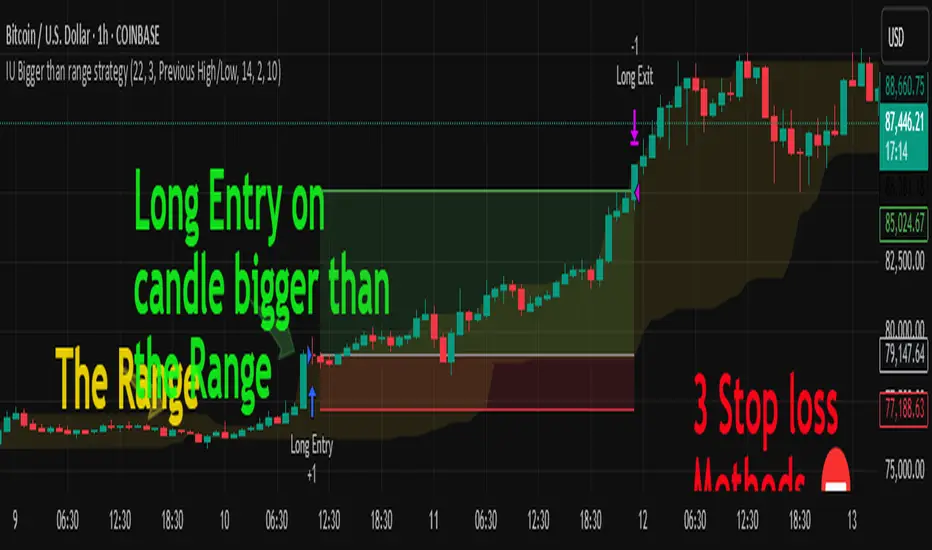
IU Bigger than range strategyDESCRIPTION
IU Bigger Than Range Strategy is designed to capture breakout opportunities by identifying candles that are significantly larger than the previous range. It dynamically calculates the high and low of the last N candles and enters trades when the current candle's range exceeds the previous range. The strategy includes multiple stop-loss methods (Previous High/Low, ATR, Swing High/Low) and automatically manages take-profit and stop-loss levels based on user-defined risk-to-reward ratios. This versatile strategy is optimized for higher timeframes and assets like BTC but can be fine-tuned for different instruments and intervals.
USER INPUTS:
Look back Length: Number of candles to calculate the high-low range. Default is 22.
Risk to Reward: Sets the target reward relative to the stop-loss distance. Default is 3.
Stop Loss Method: Choose between:(Default is "Previous High/Low")
- Previous High/Low
- ATR (Average True Range)
- Swing High/Low
ATR Length: Defines the length for ATR calculation (only applicable when ATR is selected as the stop-loss method) (Default is 14).
ATR Factor: Multiplier applied to the ATR to determine stop-loss distance(Default is 2).
Swing High/Low Length: Specifies the length for identifying swing points (only applicable when Swing High/Low is selected as the stop-loss method).(Default is 2)
LONG CONDITION:
The current candle’s range (absolute difference between open and close) is greater than the previous range.
The closing price is higher than the opening price (bullish candle).
SHORT CONDITIONS:
The current candle’s range exceeds the previous range.
The closing price is lower than the opening price (bearish candle).
LONG EXIT:
Stop-loss:
- Previous Low
- ATR-based trailing stop
- Recent Swing Low
Take-profit:
- Defined by the Risk-to-Reward ratio (default 3x the stop-loss distance).
SHORT EXIT:
Stop-loss:
- Previous High
- ATR-based trailing stop
- Recent Swing High
Take-profit:
- Defined by the Risk-to-Reward ratio (default 3x the stop-loss distance).
ALERTS:
Long Entry Triggered
Short Entry Triggered
WHY IT IS UNIQUE:
This strategy dynamically adapts to different market conditions by identifying candles that exceed the previous range, ensuring that it only enters trades during strong breakout scenarios.
Multiple stop-loss methods provide flexibility for different trading styles and risk profiles.
The visual representation of stop-loss and take-profit levels with color-coded plots improves trade monitoring and decision-making.
HOW USERS CAN BENEFIT FROM IT:
Ideal for breakout traders looking to capitalize on momentum-driven price moves.
Provides flexibility to customize stop-loss methods and fine-tune risk management parameters.
Helps minimize drawdowns with a strong risk-to-reward framework while maximizing profit potential.
Trendline Breaks with Multi Fibonacci Supertrend StrategyTMFS Strategy: Advanced Trendline Breakouts with Multi-Fibonacci Supertrend
Elevate your algorithmic trading with institutional-grade signal confluence
Strategy Genesis & Evolution
This advanced trading system represents the culmination of a personal research journey, evolving from my custom " Multi Fibonacci Supertrend with Signals " indicator into a comprehensive trading strategy. Built upon the exceptional trendline detection methodology pioneered by LuxAlgo in their " Trendlines with Breaks " indicator, I've engineered a systematic framework that integrates multiple technical factors into a cohesive trading system.
Core Fibonacci Principles
At the heart of this strategy lies the Fibonacci sequence application to volatility measurement:
// Fibonacci-based factors for multiple Supertrend calculations
factor1 = input.float(0.618, 'Factor 1 (Weak/Fibonacci)', minval = 0.01, step = 0.01)
factor2 = input.float(1.618, 'Factor 2 (Medium/Golden Ratio)', minval = 0.01, step = 0.01)
factor3 = input.float(2.618, 'Factor 3 (Strong/Extended Fib)', minval = 0.01, step = 0.01)
These precise Fibonacci ratios create a dynamic volatility envelope that adapts to changing market conditions while maintaining mathematical harmony with natural price movements.
Dynamic Trendline Detection
The strategy incorporates LuxAlgo's pioneering approach to trendline detection:
// Pivotal swing detection (inspired by LuxAlgo)
pivot_high = ta.pivothigh(swing_length, swing_length)
pivot_low = ta.pivotlow(swing_length, swing_length)
// Dynamic slope calculation using ATR
slope = atr_value / swing_length * atr_multiplier
// Update trendlines based on pivot detection
if bool(pivot_high)
upper_slope := slope
upper_trendline := pivot_high
else
upper_trendline := nz(upper_trendline) - nz(upper_slope)
This adaptive trendline approach automatically identifies key structural market boundaries, adjusting in real-time to evolving chart patterns.
Breakout State Management
The strategy implements sophisticated state tracking for breakout detection:
// Track breakouts with state variables
var int upper_breakout_state = 0
var int lower_breakout_state = 0
// Update breakout state when price crosses trendlines
upper_breakout_state := bool(pivot_high) ? 0 : close > upper_trendline ? 1 : upper_breakout_state
lower_breakout_state := bool(pivot_low) ? 0 : close < lower_trendline ? 1 : lower_breakout_state
// Detect new breakouts (state transitions)
bool new_upper_breakout = upper_breakout_state > upper_breakout_state
bool new_lower_breakout = lower_breakout_state > lower_breakout_state
This state-based approach enables precise identification of the exact moment when price breaks through a significant trendline.
Multi-Factor Signal Confluence
Entry signals require confirmation from multiple technical factors:
// Define entry conditions with multi-factor confluence
long_entry_condition = enable_long_positions and
upper_breakout_state > upper_breakout_state and // New trendline breakout
di_plus > di_minus and // Bullish DMI confirmation
close > smoothed_trend // Price above Supertrend envelope
// Execute trades only with full confirmation
if long_entry_condition
strategy.entry('L', strategy.long, comment = "LONG")
This strict requirement for confluence significantly reduces false signals and improves the quality of trade entries.
Advanced Risk Management
The strategy includes sophisticated risk controls with multiple methodologies:
// Calculate stop loss based on selected method
get_long_stop_loss_price(base_price) =>
switch stop_loss_method
'PERC' => base_price * (1 - long_stop_loss_percent)
'ATR' => base_price - long_stop_loss_atr_multiplier * entry_atr
'RR' => base_price - (get_long_take_profit_price() - base_price) / long_risk_reward_ratio
=> na
// Implement trailing functionality
strategy.exit(
id = 'Long Take Profit / Stop Loss',
from_entry = 'L',
qty_percent = take_profit_quantity_percent,
limit = trailing_take_profit_enabled ? na : long_take_profit_price,
stop = long_stop_loss_price,
trail_price = trailing_take_profit_enabled ? long_take_profit_price : na,
trail_offset = trailing_take_profit_enabled ? long_trailing_tp_step_ticks : na,
comment = "TP/SL Triggered"
)
This flexible approach adapts to varying market conditions while providing comprehensive downside protection.
Performance Characteristics
Rigorous backtesting demonstrates exceptional capital appreciation potential with impressive risk-adjusted metrics:
Remarkable total return profile (1,517%+)
Strong Sortino ratio (3.691) indicating superior downside risk control
Profit factor of 1.924 across all trades (2.153 for long positions)
Win rate exceeding 35% with balanced distribution across varied market conditions
Institutional Considerations
The strategy architecture addresses execution complexities faced by institutional participants with temporal filtering and date-range capabilities:
// Time Filter settings with flexible timezone support
import jason5480/time_filters/5 as time_filter
src_timezone = input.string(defval = 'Exchange', title = 'Source Timezone')
dst_timezone = input.string(defval = 'Exchange', title = 'Destination Timezone')
// Date range filtering for precise execution windows
use_from_date = input.bool(defval = true, title = 'Enable Start Date')
from_date = input.time(defval = timestamp('01 Jan 2022 00:00'), title = 'Start Date')
// Validate trading permission based on temporal constraints
date_filter_approved = time_filter.is_in_date_range(
use_from_date, from_date, use_to_date, to_date, src_timezone, dst_timezone
)
These capabilities enable precise execution timing and market session optimization critical for larger market participants.
Acknowledgments
Special thanks to LuxAlgo for the pioneering work on trendline detection and breakout identification that inspired elements of this strategy. Their innovative approach to technical analysis provided a valuable foundation upon which I could build my Fibonacci-based methodology.
This strategy is shared under the same Attribution-NonCommercial-ShareAlike 4.0 International (CC BY-NC-SA 4.0) license as LuxAlgo's original work.
Past performance is not indicative of future results. Conduct thorough analysis before implementing any algorithmic strategy.

BTCUSD with adjustable sl,tpThis strategy is designed for swing traders who want to enter long positions on pullbacks after a short-term trend shift, while also allowing immediate short entries when conditions favor downside movement. It combines SMA crossovers, a fixed-percentage retracement entry, and adjustable risk management parameters for optimal trade execution.
Key Features:
✅ Trend Confirmation with SMA Crossover
The 10-period SMA crossing above the 25-period SMA signals a bullish trend shift.
The 10-period SMA crossing below the 25-period SMA signals a bearish trend shift.
Short trades are only taken if the price is below the 150 EMA, ensuring alignment with the broader trend.
📉 Long Pullback Entry Using Fixed Percentage Retracement
Instead of entering immediately on the SMA crossover, the strategy waits for a retracement before going long.
The pullback entry is defined as a percentage retracement from the recent high, allowing for an optimized entry price.
The retracement percentage is fully adjustable in the settings (default: 1%).
A dynamic support level is plotted on the chart to visualize the pullback entry zone.
📊 Short Entry Rules
If the SMA(10) crosses below the SMA(25) and price is below the 150 EMA, a short trade is immediately entered.
Risk Management & Exit Strategy:
🚀 Take Profit (TP) – Fully customizable profit target in points. (Default: 1000 points)
🛑 Stop Loss (SL) – Adjustable stop loss level in points. (Default: 250 points)
🔄 Break-Even (BE) – When price moves in favor by a set number of points, the stop loss is moved to break-even.
📌 Extra Exit Condition for Longs:
If the SMA(10) crosses below SMA(25) while the price is still below the EMA150, the strategy force-exits the long position to avoid reversals.
How to Use This Strategy:
Enable the strategy on your TradingView chart (recommended for stocks, forex, or indices).
Customize the settings – Adjust TP, SL, BE, and pullback percentage for your risk tolerance.
Observe the plotted retracement levels – When the price touches and bounces off the level, a long trade is triggered.
Let the strategy manage the trade – Break-even protection and take-profit logic will automatically execute.
Ideal Market Conditions:
✅ Trending Markets – The strategy works best when price follows strong trends.
✅ Stocks, Indices, or Forex – Can be applied across multiple asset classes.
✅ Medium-Term Holding Period – Suitable for swing trades lasting days to weeks.

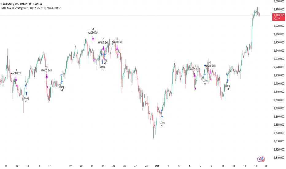
Multi-Timeframe MACD Strategy ver 1.0Multi-Timeframe MACD Strategy: Enhanced Trend Trading with Customizable Entry and Trailing Stop
This strategy utilizes the Moving Average Convergence Divergence (MACD) indicator across multiple timeframes to identify strong trends, generate precise entry and exit signals, and manage risk with an optional trailing stop loss. By combining the insights of both the current chart's timeframe and a user-defined higher timeframe, this strategy aims to improve trade accuracy, reduce exposure to false signals, and capture larger market moves.
Key Features:
Dual Timeframe Analysis: Calculates and analyzes the MACD on both the current chart's timeframe and a user-selected higher timeframe (e.g., Daily MACD on a 1-hour chart). This provides a broader market context, helping to confirm trends and filter out short-term noise.
Configurable MACD: Fine-tune the MACD calculation with adjustable Fast Length, Slow Length, and Signal Length parameters. Optimize the indicator's sensitivity to match your trading style and the volatility of the asset.
Flexible Entry Options: Choose between three distinct entry types:
Crossover: Enters trades when the MACD line crosses above (long) or below (short) the Signal line.
Zero Cross: Enters trades when the MACD line crosses above (long) or below (short) the zero line.
Both: Combines both Crossover and Zero Cross signals, providing more potential entry opportunities.
Independent Timeframe Control: Display and trade based on the current timeframe MACD, the higher timeframe MACD, or both. This allows you to focus on the information most relevant to your analysis.
Optional Trailing Stop Loss: Implements a configurable trailing stop loss to protect profits and limit potential losses. The trailing stop is adjusted dynamically as the price moves in your favor, based on a user-defined percentage.
No Repainting: Employs lookahead=barmerge.lookahead_off in the request.security() function to prevent data leakage and ensure accurate backtesting and real-time signals.
Clear Visual Signals (Optional): Includes optional plotting of the MACD and Signal lines for both timeframes, with distinct colors for easy visual identification. These plots are for visual confirmation and are not required for the strategy's logic.
Suitable for Various Trading Styles: Adaptable to swing trading, day trading, and trend-following strategies across diverse markets (stocks, forex, cryptocurrencies, etc.).
Fully Customizable: All parameters are adjustable, including timeframes, MACD Settings, Entry signal type and trailing stop settings.
How it Works:
MACD Calculation: The strategy calculates the MACD (using the standard formula) for both the current chart's timeframe and the specified higher timeframe.
Trend Identification: The relationship between the MACD line, Signal line, and zero line is used to determine the current trend for each timeframe.
Entry Signals: Buy/sell signals are generated based on the selected "Entry Type":
Crossover: A long signal is generated when the MACD line crosses above the Signal line, and both timeframes are in agreement (if both are enabled). A short signal is generated when the MACD line crosses below the Signal line, and both timeframes are in agreement.
Zero Cross: A long signal is generated when the MACD line crosses above the zero line, and both timeframes agree. A short signal is generated when the MACD line crosses below the zero line and both timeframes agree.
Both: Combines Crossover and Zero Cross signals.
Trailing Stop Loss (Optional): If enabled, a trailing stop loss is set at a specified percentage below (for long positions) or above (for short positions) the entry price. The stop-loss is automatically adjusted as the price moves favorably.
Exit Signals:
Without Trailing Stop: Positions are closed when the MACD signals reverse according to the selected "Entry Type" (e.g., a long position is closed when the MACD line crosses below the Signal line if using "Crossover" entries).
With Trailing Stop: Positions are closed if the price hits the trailing stop loss.
Backtesting and Optimization: The strategy automatically backtests on the chart's historical data, allowing you to assess its performance and optimize parameters for different assets and timeframes.
Example Use Cases:
Confirming Trend Strength: A trader on a 1-hour chart sees a bullish MACD crossover on the current timeframe. They check the MTF MACD strategy and see that the Daily MACD is also bullish, confirming the strength of the uptrend.
Filtering Noise: A trader using a 15-minute chart wants to avoid false signals from short-term volatility. They use the strategy with a 4-hour higher timeframe to filter out noise and only trade in the direction of the dominant trend.
Dynamic Risk Management: A trader enters a long position and enables the trailing stop loss. As the price rises, the trailing stop is automatically adjusted upwards, protecting profits. The trade is exited either when the MACD reverses or when the price hits the trailing stop.
Disclaimer:
The MACD is a lagging indicator and can produce false signals, especially in ranging markets. This strategy is for educational and informational purposes only and should not be considered financial advice. Backtest and optimize the strategy thoroughly, combine it with other technical analysis tools, and always implement sound risk management practices before using it with real capital. Past performance is not indicative of future results. Conduct your own due diligence and consider your risk tolerance before making any trading decisions.
Multi-Timeframe Parabolic SAR Strategy ver 1.0Multi-Timeframe Parabolic SAR Strategy (MTF PSAR) - Enhanced Trend Trading
This strategy leverages the power of the Parabolic SAR (Stop and Reverse) indicator across multiple timeframes to provide robust trend identification, precise entry/exit signals, and dynamic trailing stop management. By combining the insights of both the current chart's timeframe and a user-defined higher timeframe, this strategy aims to improve trading accuracy, reduce risk, and capture more significant market moves.
Key Features:
Dual Timeframe Analysis: Simultaneously analyzes the Parabolic SAR on the current chart and a higher timeframe (e.g., Daily PSAR on a 1-hour chart). This allows you to align your trades with the dominant trend and filter out noise from lower timeframes.
Configurable PSAR: Fine-tune the PSAR calculation with adjustable Start, Increment, and Maximum values to optimize sensitivity for your trading style and the asset's volatility.
Independent Timeframe Control: Choose to display and trade based on either or both the current timeframe PSAR and the higher timeframe PSAR. Focus on the most relevant information for your analysis.
Clear Visual Signals: Distinct colors for the current and higher timeframe PSAR dots provide a clear visual representation of potential entry and exit points.
Multiple Entry Strategies: The strategy offers flexible entry conditions, allowing you to trade based on:
Confirmation: Both current and higher timeframe PSAR signals agree and the current timeframe PSAR has just flipped direction. (Most conservative)
Current Timeframe Only: Trades based solely on the current timeframe PSAR, ideal for when the higher timeframe is less relevant or disabled.
Higher Timeframe Only: Trades based solely on the higher timeframe PSAR.
Dynamic Trailing Stop (PSAR-Based): Implements a trailing stop-loss based on the current timeframe's Parabolic SAR. This helps protect profits by automatically adjusting the stop-loss as the price moves in your favor. Exits are triggered when either the current or HTF PSAR flips.
No Repainting: Uses lookahead=barmerge.lookahead_off in the security() function to ensure that the higher timeframe data is accessed without any data leakage, preventing repainting issues.
Fully Configurable: All parameters (PSAR settings, higher timeframe, visibility, colors) are adjustable through the strategy's settings panel, allowing for extensive customization and optimization.
Suitable for Various Trading Styles: Applicable to swing trading, day trading, and trend-following strategies across various markets (stocks, forex, cryptocurrencies, etc.).
How it Works:
PSAR Calculation: The strategy calculates the standard Parabolic SAR for both the current chart's timeframe and the selected higher timeframe.
Trend Identification: The direction of the PSAR (dots below price = uptrend, dots above price = downtrend) determines the current trend for each timeframe.
Entry Signals: The strategy generates buy/sell signals based on the chosen entry strategy (Confirmation, Current Timeframe Only, or Higher Timeframe Only). The Confirmation strategy offers the highest probability signals by requiring agreement between both timeframes.
Trailing Stop Exit: Once a position is entered, the strategy uses the current timeframe PSAR as a dynamic trailing stop. The stop-loss is automatically adjusted as the PSAR dots move, helping to lock in profits and limit losses. The strategy exits when either the Current or HTF PSAR changes direction.
Backtesting and Optimization: The strategy automatically backtests on the chart's historical data, allowing you to evaluate its performance and optimize the settings for different assets and timeframes.
Example Use Cases:
Trend Confirmation: A trader on a 1-hour chart observes a bullish PSAR flip on the current timeframe. They check the MTF PSAR strategy and see that the Daily PSAR is also bullish, confirming the strength of the uptrend and providing a high-probability long entry signal.
Filtering Noise: A trader on a 5-minute chart wants to avoid whipsaws caused by short-term price fluctuations. They use the strategy with a 1-hour higher timeframe to filter out noise and only trade in the direction of the dominant trend.
Dynamic Risk Management: A trader enters a long position and uses the current timeframe PSAR as a trailing stop. As the price rises, the PSAR dots move upwards, automatically raising the stop-loss and protecting profits. The trade is exited when the current (or HTF) PSAR flips to bearish.
Disclaimer:
The Parabolic SAR is a lagging indicator and can produce false signals, particularly in ranging or choppy markets. This strategy is intended for educational and informational purposes only and should not be considered financial advice. It is essential to backtest and optimize the strategy thoroughly, use it in conjunction with other technical analysis tools, and implement sound risk management practices before using it with real capital. Past performance is not indicative of future results. Always conduct your own due diligence and consider your risk tolerance before making any trading decisions.

IU Gap Fill StrategyThe IU Gap Fill Strategy is designed to capitalize on price gaps that occur between trading sessions. It identifies gaps based on a user-defined percentage threshold and executes trades when the price fills the gap within a day. This strategy is ideal for traders looking to take advantage of market inefficiencies that arise due to overnight or session-based price movements. An ATR-based trailing stop-loss is incorporated to dynamically manage risk and lock in profits.
USER INPUTS
Percentage Difference for Valid Gap - Defines the minimum gap size in percentage terms for a valid trade setup. ( Default is 0.2 )
ATR Length - Sets the lookback period for the Average True Range (ATR) calculation. (default is 14 )
ATR Factor - Determines the multiplier for the trailing stop-loss, helping in risk management. ( Default is 2.00 )
LONG CONDITION
A gap-up occurs, meaning the current session opens above the previous session’s close.
The price initially dips below the previous session's close but then recovers and closes above it.
The gap meets the valid percentage threshold set by the user.
The bar is not the first or last bar of the session to avoid false signals.
SHORT CONDITION
A gap-down occurs, meaning the current session opens below the previous session’s close.
The price initially moves above the previous session’s close but then closes below it.
The gap meets the valid percentage threshold set by the user.
The bar is not the first or last bar of the session to avoid false signals.
LONG EXIT
An ATR-based trailing stop-loss is set below the entry price and dynamically adjusts upwards as the price moves in favor of the trade.
The position is closed when the trailing stop-loss is hit.
SHORT EXIT
An ATR-based trailing stop-loss is set above the entry price and dynamically adjusts downwards as the price moves in favor of the trade.
The position is closed when the trailing stop-loss is hit.
WHY IT IS UNIQUE
Precision in Identifying Gaps - The strategy focuses on real price gaps rather than minor fluctuations.
Dynamic Risk Management - Uses ATR-based trailing stop-loss to secure profits while allowing the trade to run.
Versatility - Works on stocks, indices, forex, and any market that experiences session-based gaps.
Optimized Entry Conditions - Ensures entries are taken only when the price attempts to fill the gap, reducing false signals.
HOW USERS CAN BENEFIT FROM IT
Enhance Trade Timing - Captures high-probability trade setups based on market inefficiencies caused by gaps.
Minimize Risk - The ATR trailing stop-loss helps protect gains and limit losses.
Works in Different Market Conditions - Whether markets are trending or consolidating, the strategy adapts to potential gap fill opportunities.
Fully Customizable - Users can fine-tune gap percentage, ATR settings, and stop-loss parameters to match their trading style.

Dual SuperTrend w VIX Filter - Strategy [presentTrading]Hey everyone! Haven't been here for a long time. Been so busy again in the past 2 months. I recently started working on analyzing the combination of trend strategy and VIX, but didn't get outstanding results after a few tries. Sharing this tool with all of you in case you have better insights.
█ Introduction and How it is Different
The Dual SuperTrend with VIX Filter Strategy combines traditional trend following with market volatility analysis. Unlike conventional SuperTrend strategies that focus solely on price action, this experimental system incorporates VIX (Volatility Index) as an adaptive filter to create a more context-aware trading approach. By analyzing where current volatility stands relative to historical norms, the strategy adjusts to different market environments rather than applying uniform logic across all conditions.
BTCUSD 6hr Long Short Performance
█ Strategy, How it Works: Detailed Explanation
🔶 Dual SuperTrend Core
The strategy uses two SuperTrend indicators with different sensitivity settings:
- SuperTrend 1: Length = 13, Multiplier = 3.5
- SuperTrend 2: Length = 8, Multiplier = 5.0
The SuperTrend calculation follows this process:
1. ATR = Average of max(High-Low, |High-PreviousClose|, |Low-PreviousClose|) over 'length' periods
2. UpperBand = (High+Low)/2 - (Multiplier * ATR)
3. LowerBand = (High+Low)/2 + (Multiplier * ATR)
Trend direction is determined by:
- If Close > previous LowerBand, Trend = Bullish (1)
- If Close < previous UpperBand, Trend = Bearish (-1)
- Otherwise, Trend = previous Trend
🔶 VIX Analysis Framework
The core innovation lies in the VIX analysis system:
1. Statistical Analysis:
- VIX Mean = SMA(VIX, 252)
- VIX Standard Deviation = StdDev(VIX, 252)
- VIX Z-Score = (Current VIX - VIX Mean) / VIX StdDev
2. **Volatility Bands:
- Upper Band 1 = VIX Mean + (2 * VIX StdDev)
- Upper Band 2 = VIX Mean + (3 * VIX StdDev)
- Lower Band 1 = VIX Mean - (2 * VIX StdDev)
- Lower Band 2 = VIX Mean - (3 * VIX StdDev)
3. Volatility Regimes:
- "Very Low Volatility": VIX < Lower Band 1
- "Low Volatility": Lower Band 1 ≤ VIX < Mean
- "Normal Volatility": Mean ≤ VIX < Upper Band 1
- "High Volatility": Upper Band 1 ≤ VIX < Upper Band 2
- "Extreme Volatility": VIX ≥ Upper Band 2
4. VIX Trend Detection:
- VIX EMA = EMA(VIX, 10)
- VIX Rising = VIX > VIX EMA
- VIX Falling = VIX < VIX EMA
Local performance:
🔶 Entry Logic Integration
The strategy combines trend signals with volatility filtering:
Long Entry Condition:
- Both SuperTrend 1 AND SuperTrend 2 must be bullish (trend = 1)
- AND selected VIX filter condition must be satisfied
Short Entry Condition:
- Both SuperTrend 1 AND SuperTrend 2 must be bearish (trend = -1)
- AND selected VIX filter condition must be satisfied
Available VIX filter rules include:
- "Below Mean + SD": VIX < Lower Band 1
- "Below Mean": VIX < VIX Mean
- "Above Mean": VIX > VIX Mean
- "Above Mean + SD": VIX > Upper Band 1
- "Falling VIX": VIX < VIX EMA
- "Rising VIX": VIX > VIX EMA
- "Any": No VIX filtering
█ Trade Direction
The strategy allows testing in three modes:
1. **Long Only:** Test volatility effects on uptrends only
2. **Short Only:** Examine volatility's impact on downtrends only
3. **Both (Default):** Compare how volatility affects both trend directions
This enables comparative analysis of how volatility regimes impact bullish versus bearish markets differently.
█ Usage
Use this strategy as an experimental framework:
1. Form a hypothesis about how volatility affects trend reliability
2. Configure VIX filters to test your specific hypothesis
3. Analyze performance across different volatility regimes
4. Compare results between uptrends and downtrends
5. Refine your volatility filtering approach based on results
6. Share your findings with the trading community
This framework allows you to investigate questions like:
- Are uptrends more reliable during rising or falling volatility?
- Do downtrends perform better when volatility is above or below its historical average?
- Should different volatility filters be applied to long vs. short positions?
█ Default Settings
The default settings serve as a starting point for exploration:
SuperTrend Parameters:
- SuperTrend 1 (Length=13, Multiplier=3.5): More responsive to trend changes
- SuperTrend 2 (Length=8, Multiplier=5.0): More selective filter requiring stronger trends
VIX Analysis Settings:
- Lookback Period = 252: Establishes a full market cycle for volatility context
- Standard Deviation Bands = 2 and 3 SD: Creates statistically significant regime boundaries
- VIX Trend Period = 10: Balances responsiveness with noise reduction
Default VIX Filter Selection:
- Long Entry: "Above Mean" - Tests if uptrends perform better during above-average volatility
- Short Entry: "Rising VIX" - Tests if downtrends accelerate when volatility is increasing
Feel Free to share your insight below!!!

Double Bollinger Bands Strategy with Signals (By Rolwin)Double Bollinger Bands Strategy with Signals 1.0 (By Rolwin)
📌 Overview
The Double Bollinger Bands Strategy is a trend-following system that utilizes two sets of Bollinger Bands (2 standard deviations and 3 standard deviations) to identify high-probability entry and exit points. This strategy helps traders capitalize on strong price movements and potential reversals by detecting overbought and oversold conditions more effectively.
📊 How It Works
• Bollinger Bands Setup:
o Middle Band: 20-period Simple Moving Average (SMA)
o Upper & Lower Bands (2 SD): Standard Bollinger Bands (±2 standard deviations)
o Extreme Bands (3 SD): Additional Bollinger Bands (±3 standard deviations) for extreme price moves
• Entry Signals:
✅ Buy (Long Entry): When the price crosses above the lower 3SD band (oversold zone)
❌ Sell (Short Entry): When the price crosses below the upper 3SD band (overbought zone)
• Exit Signals:
🔼 Exit Long: When the price reaches the upper 2SD band
🔽 Exit Short: When the price reaches the lower 2SD band
• Additional Features:
✅ Buy & Sell Signals plotted directly on the chart
🎨 Candles turn white when price touches the extreme 3SD band
🔥 Why Use This Strategy?
✔️ Clear Entry & Exit Points: Based on strong statistical levels
✔️ Effective in Trending & Reversal Markets: Captures both momentum & mean reversion setups
✔️ Easy-to-Use Visualization: Signals & bands make it beginner-friendly
✔️ Customizable: Adjust Bollinger Band length and multipliers to fit different assets & timeframes
⚠️ Risk Management Tip
While this strategy provides high-probability trade signals, it is essential to use stop-loss orders (e.g., ATR-based) and proper position sizing to manage risk effectively.
📈 Try it out and optimize the settings for your favorite markets! 🚀

Strategy SuperTrend SDI WebhookThis Pine Script™ strategy is designed for automated trading in TradingView. It combines the SuperTrend indicator and Smoothed Directional Indicator (SDI) to generate buy and sell signals, with additional risk management features like stop loss, take profit, and trailing stop. The script also includes settings for leverage trading, equity-based position sizing, and webhook integration.
Key Features
1. Date-based Trade Execution
The strategy is active only between the start and end dates set by the user.
times ensures that trades occur only within this predefined time range.
2. Position Sizing and Leverage
Uses leverage trading to adjust position size dynamically based on initial equity.
The user can set leverage (leverage) and percentage of equity (usdprcnt).
The position size is calculated dynamically (initial_capital) based on account performance.
3. Take Profit, Stop Loss, and Trailing Stop
Take Profit (tp): Defines the target profit percentage.
Stop Loss (sl): Defines the maximum allowable loss per trade.
Trailing Stop (tr): Adjusts dynamically based on trade performance to lock in profits.
4. SuperTrend Indicator
SuperTrend (ta.supertrend) is used to determine the market trend.
If the price is above the SuperTrend line, it indicates an uptrend (bullish).
If the price is below the SuperTrend line, it signals a downtrend (bearish).
Plots visual indicators (green/red lines and circles) to show trend changes.
5. Smoothed Directional Indicator (SDI)
SDI helps to identify trend strength and momentum.
It calculates +DI (bullish strength) and -DI (bearish strength).
If +DI is higher than -DI, the market is considered bullish.
If -DI is higher than +DI, the market is considered bearish.
The background color changes based on the SDI signal.
6. Buy & Sell Conditions
Long Entry (Buy) Conditions:
SDI confirms an uptrend (+DI > -DI).
SuperTrend confirms an uptrend (price crosses above the SuperTrend line).
Short Entry (Sell) Conditions:
SDI confirms a downtrend (+DI < -DI).
SuperTrend confirms a downtrend (price crosses below the SuperTrend line).
Optionally, trades can be filtered using crossovers (occrs option).
7. Trade Execution and Exits
Market entries:
Long (strategy.entry("Long")) when conditions match.
Short (strategy.entry("Short")) when bearish conditions are met.
Trade exits:
Uses predefined take profit, stop loss, and trailing stop levels.
Positions are closed if the strategy is out of the valid time range.
Usage
Automated Trading Strategy:
Can be integrated with webhooks for automated execution on supported trading platforms.
Trend-Following Strategy:
Uses SuperTrend & SDI to identify trend direction and strength.
Risk-Managed Leverage Trading:
Supports position sizing, stop losses, and trailing stops.
Backtesting & Optimization:
Can be used for historical performance analysis before deploying live.
Conclusion
This strategy is suitable for traders who want to automate their trading using SuperTrend and SDI indicators. It incorporates risk management tools like stop loss, take profit, and trailing stop, making it adaptable for leverage trading. Traders can customize settings, conduct backtests, and integrate it with webhooks for real-time trade execution. 🚀
Important Note:
This script is provided for educational and template purposes and does not constitute financial advice. Traders and investors should conduct their research and analysis before making any trading decisions.

Supertrend Strategy with Money Ocean TradeStrategy Overview
The Supertrend Strategy with Trend Change Confirmation leverages the Supertrend indicator to identify potential buy and sell signals based on changes in trend direction and subsequent price action. The strategy is designed to work with any financial instrument (symbol) and aims to provide clear entry and exit signals.
Key Components
Supertrend Indicator: The core of this strategy is the Supertrend indicator, calculated using a length of 3 and a factor of 1. The Supertrend line is plotted on the chart to visually represent trend direction.
Direction 1: Indicates an uptrend (bullish).
Direction -1: Indicates a downtrend (bearish).
Trend Change Detection: The strategy monitors changes in the trend direction. When a trend change is detected, it checks if the next candle confirms the trend change by breaking above or below the Supertrend line.
Entry Conditions:
Long Entry (Buy): When the Supertrend direction changes to 1 (uptrend) and the next candle closes above the Supertrend line.
Short Entry (Sell): When the Supertrend direction changes to -1 (downtrend) and the next candle closes below the Supertrend line.
Exit Conditions: The strategy closes the position based on the opposite signal.
Long Exit: When the Supertrend direction changes to -1 (downtrend) and the next candle closes below the Supertrend line.
Short Exit: When the Supertrend direction changes to 1 (uptrend) and the next candle closes above the Supertrend line.
Visual Signals: The strategy plots buy and sell signals on the chart using plotshape:
BUY: A green label below the bar when a long entry is triggered.
SELL: A red label above the bar when a short entry is triggered.
Alerts: Alerts are set up to notify when a buy or sell signal is triggered.
Script Summary
This strategy helps traders identify potential trading opportunities based on trend changes and confirms the trend by checking the next candle's price action. The visual signals and dashboard enhance the user's ability to monitor and manage trades effectively.
Feel free to test and adjust the parameters to suit your trading preferences! If you need further customizations or explanations, let me know.

Boilerplate Configurable Strategy [Yosiet]This is a Boilerplate Code!
Hello! First of all, let me introduce myself a little bit. I don't come from the world of finance, but from the world of information and communication technologies (ICT) where we specialize in data processing with the aim of automating it and eliminating all human factors and actors in the processes. You could say that I am an algotrader.
That said, in my journey through trading in recent years I have understood that this world is often shown to be incomplete. All those who want to learn about trading only end up learning a small part of what it really entails, they only seek to learn how to read candlesticks. Therefore, I want to share with the entire community a fraction of what I have really understood it to be.
As a computer scientist, the most important thing is the data, it is the raw material of our work and without data you simply cannot do anything. Entropy is simple: Data in -> Data is transformed -> Data out.
The quality of the outgoing data will directly depend on the incoming data, there is no greater mystery or magic in the process. In trading it is no different, because at the end of the day it is nothing more than data. As we often say, if garbage comes in, garbage comes out.
Most people focus on the results only, on the outgoing data, because in the end we all want the same thing, to make easy money. Very few pay attention to the input data, much less to the process.
Now, I am not here to delude you, because there is no bigger lie than easy money, but I am here to give you a boilerplate code that will help you create strategies where you only have to concentrate on the quality of the incoming data.
To the Point
The code is a strategy boilerplate that applies the technique that you decide to customize for the criteria for opening a position. It already has the other factors involved in trading programmed and automated.
1. The Entry
This section of the boilerplate is the one that each individual must customize according to their needs and knowledge. The code is offered with two simple, well-known strategies to exemplify how the code can be reused for your own benefits.
For the purposes of this post on tradingview, I am going to use the simplest of the known strategies in trading for entries: SMA Crossing
// SMA Cross Settings
maFast = ta.sma(close, length)
maSlow = ta.sma(open, length)
The Strategy Properties for all cases published here:
For Stock TSLA H1 From 01/01/2025 To 02/15/2025
For Crypto XMR-USDT 30m From 01/01/2025 To 02/15/2025
For Forex EUR-USD 5m From 01/01/2025 To 02/15/2025
But the goal of this post is not to sell you a dream, else to show you that the same Entry decision works very well for some and does not for others and with this boilerplate code you only have to think of entries, not exits.
2. Schedules, Days, Sessions
As you know, there are an infinite number of markets that are susceptible to the sessions of each country and the news that they announce during those sessions, so the code already offers parameters so that you can condition the days and hours of operation, filter the best time parameters for a specific market and time frame.
3. Data Filtering
The data offered in trading are numerical series presented in vectors on a time axis where an endless number of mathematical equations can be applied to process them, with matrix calculation and non-linear regressions being the best, in my humble opinion.
4. Read Fundamental Macroeconomic Events, News
The boilerplate has integration with the tradingview SDK to detect when news will occur and offers parameters so that you can enable an exclusion time margin to not operate anything during that time window.
5. Direction and Sense
In my experience I have found the peculiarity that the same algorithm works very well for a market in a time frame, but for the same market in another time frame it is only a waste of time and money. So now you can easily decide if you only want to open LONG, SHORT or both side positions and know how effective your strategy really is.
6. Reading the money, THE PURPOSE OF EVERYTHING
The most important section in trading and the reason why many clients usually hire me as a financial programmer, is reading and controlling the money, because in the end everyone wants to win and no one wants to lose. Now they can easily parameterize how the money should flow and this is the genius of this boilerplate, because it is what will really decide if an algorithm (Indicator: A bunch of math equations) for entries will really leave you good money over time.
7. Managing the Risk, The Ego Destroyer
Many trades, little money. Most traders focus on making money and none of them know about statistics and the few who do know something about it, only focus on the winrate. Well, with this code you can unlock what really matters, the true success criteria to be able to live off of trading: Profit Factor, Sortino Ratio, Sharpe Ratio and most importantly, will you really make money?
8. Managing Emotions
Finally, the main reason why many lose money is because they are very bad at managing their emotions, because with this they will no longer need to do so because the boilerplate has already programmed criteria to chase the price in a position, cut losses and maximize profits.
In short, this is a boilerplate code that already has the data processing and data output ready, you only have to worry about the data input.
“And so the trader learned: the greatest edge was not in predicting the storm, but in building a boat that could not sink.”
DISCLAIMER
This post is intended for programmers and quantitative traders who already have a certain level of knowledge and experience. It is not intended to be financial advice or to sell you any money-making script, if you use it, you do so at your own risk.

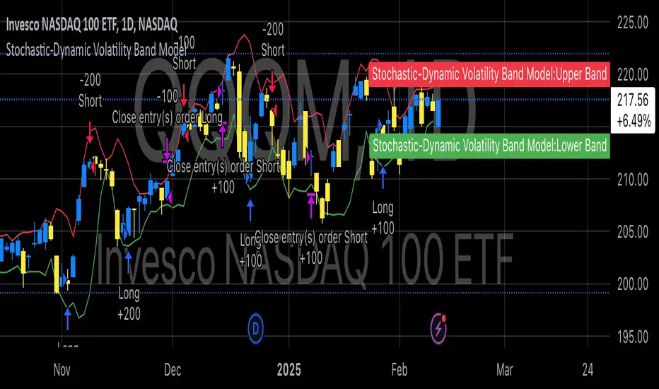
Stochastic-Dynamic Volatility Band ModelThe Stochastic-Dynamic Volatility Band Model is a quantitative trading approach that leverages statistical principles to model market volatility and generate buy and sell signals. The strategy is grounded in the concepts of volatility estimation and dynamic market regimes, where the core idea is to capture price fluctuations through stochastic models and trade around volatility bands.
Volatility Estimation and Band Construction
The volatility bands are constructed using a combination of historical price data and statistical measures, primarily the standard deviation (σ) of price returns, which quantifies the degree of variation in price movements over a specific period. This methodology is based on the classical works of Black-Scholes (1973), which laid the foundation for using volatility as a core component in financial models. Volatility is a crucial determinant of asset pricing and risk, and it plays a pivotal role in this strategy's design.
Entry and Exit Conditions
The entry conditions are based on the price’s relationship with the volatility bands. A long entry is triggered when the price crosses above the lower volatility band, indicating that the market may have been oversold or is experiencing a reversal to the upside. Conversely, a short entry is triggered when the price crosses below the upper volatility band, suggesting overbought conditions or a potential market downturn.
These entry signals are consistent with the mean reversion theory, which asserts that asset prices tend to revert to their long-term average after deviating from it. According to Poterba and Summers (1988), mean reversion occurs due to overreaction to news or temporary disturbances, leading to price corrections.
The exit condition is based on the number of bars that have elapsed since the entry signal. Specifically, positions are closed after a predefined number of bars, typically set to seven bars, reflecting a short-term trading horizon. This exit mechanism is in line with short-term momentum trading strategies discussed in literature, where traders capitalize on price movements within specific timeframes (Jegadeesh & Titman, 1993).
Market Adaptability
One of the key features of this strategy is its dynamic nature, as it adapts to the changing volatility environment. The volatility bands automatically adjust to market conditions, expanding in periods of high volatility and contracting when volatility decreases. This dynamic adjustment helps the strategy remain robust across different market regimes, as it is capable of identifying both trend-following and mean-reverting opportunities.
This dynamic adaptability is supported by the adaptive market hypothesis (Lo, 2004), which posits that market participants evolve their strategies in response to changing market conditions, akin to the adaptive nature of biological systems.
References:
Black, F., & Scholes, M. (1973). The Pricing of Options and Corporate Liabilities. Journal of Political Economy, 81(3), 637-654.
Bollinger, J. (1980). Bollinger on Bollinger Bands. Wiley.
Jegadeesh, N., & Titman, S. (1993). Returns to Buying Winners and Selling Losers: Implications for Stock Market Efficiency. Journal of Finance, 48(1), 65-91.
Lo, A. W. (2004). The Adaptive Markets Hypothesis: Market Efficiency from an Evolutionary Perspective. Journal of Portfolio Management, 30(5), 15-29.
Poterba, J. M., & Summers, L. H. (1988). Mean Reversion in Stock Prices: Evidence and Implications. Journal of Financial Economics, 22(1), 27-59.
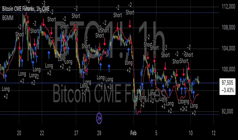
BTC Future Gamma-Weighted Momentum Model (BGMM)The BTC Future Gamma-Weighted Momentum Model (BGMM) is a quantitative trading strategy that utilizes the Gamma-weighted average price (GWAP) in conjunction with a momentum-based approach to predict price movements in the Bitcoin futures market. The model combines the concept of weighted price movements with trend identification, where the Gamma factor amplifies the weight assigned to recent prices. It leverages the idea that historical price trends and weighting mechanisms can be utilized to forecast future price behavior.
Theoretical Background:
1. Momentum in Financial Markets:
Momentum is a well-established concept in financial market theory, referring to the tendency of assets to continue moving in the same direction after initiating a trend. Any observed market return over a given time period is likely to continue in the same direction, a phenomenon known as the “momentum effect.” Deviations from a mean or trend provide potential trading opportunities, particularly in highly volatile assets like Bitcoin.
Numerous empirical studies have demonstrated that momentum strategies, based on price movements, especially those correlating long-term and short-term trends, can yield significant returns (Jegadeesh & Titman, 1993). Given Bitcoin’s volatile nature, it is an ideal candidate for momentum-based strategies.
2. Gamma-Weighted Price Strategies:
Gamma weighting is an advanced method of applying weights to price data, where past price movements are weighted by a Gamma factor. This weighting allows for the reinforcement or reduction of the influence of historical prices based on an exponential function. The Gamma factor (ranging from 0.5 to 1.5) controls how much emphasis is placed on recent data: a value closer to 1 applies an even weighting across periods, while a value closer to 0 diminishes the influence of past prices.
Gamma-based models are used in financial analysis and modeling to enhance a model’s adaptability to changing market dynamics. This weighting mechanism is particularly advantageous in volatile markets such as Bitcoin futures, as it facilitates quick adaptation to changing market conditions (Black-Scholes, 1973).
Strategy Mechanism:
The BTC Future Gamma-Weighted Momentum Model (BGMM) utilizes an adaptive weighting strategy, where the Bitcoin futures prices are weighted according to the Gamma factor to calculate the Gamma-Weighted Average Price (GWAP). The GWAP is derived as a weighted average of prices over a specific number of periods, with more weight assigned to recent periods. The calculated GWAP serves as a reference value, and trading decisions are based on whether the current market price is above or below this level.
1. Long Position Conditions:
A long position is initiated when the Bitcoin price is above the GWAP and a positive price movement is observed over the last three periods. This indicates that an upward trend is in place, and the market is likely to continue in the direction of the momentum.
2. Short Position Conditions:
A short position is initiated when the Bitcoin price is below the GWAP and a negative price movement is observed over the last three periods. This suggests that a downtrend is occurring, and a continuation of the negative price movement is expected.
Backtesting and Application to Bitcoin Futures:
The model has been tested exclusively on the Bitcoin futures market due to Bitcoin’s high volatility and strong trend behavior. These characteristics make the market particularly suitable for momentum strategies, as strong upward or downward movements are often followed by persistent trends that can be captured by a momentum-based approach.
Backtests of the BGMM on the Bitcoin futures market indicate that the model achieves above-average returns during periods of strong momentum, especially when the Gamma factor is optimized to suit the specific dynamics of the Bitcoin market. The high volatility of Bitcoin, combined with adaptive weighting, allows the model to respond quickly to price changes and maximize trading opportunities.
Scientific Citations and Sources:
• Jegadeesh, N., & Titman, S. (1993). Returns to Buying Winners and Selling Losers: Implications for Stock Market Efficiency. The Journal of Finance, 48(1), 65–91.
• Black, F., & Scholes, M. (1973). The Pricing of Options and Corporate Liabilities. Journal of Political Economy, 81(3), 637–654.
• Fama, E. F., & French, K. R. (1992). The Cross-Section of Expected Stock Returns. The Journal of Finance, 47(2), 427–465.
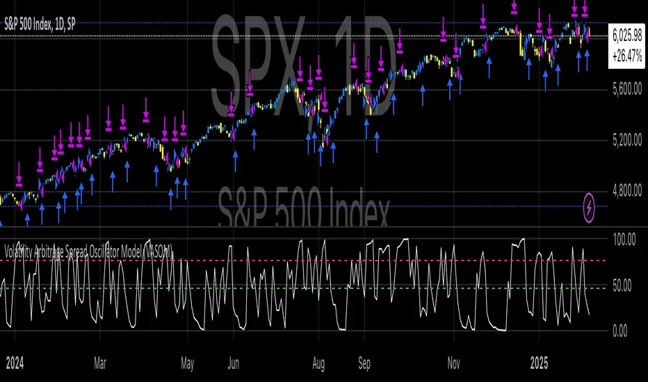
Volatility Arbitrage Spread Oscillator Model (VASOM)The Volatility Arbitrage Spread Oscillator Model (VASOM) is a systematic approach to capitalizing on price inefficiencies in the VIX futures term structure. By analyzing the differential between front-month and second-month VIX futures contracts, we employ a momentum-based oscillator (Relative Strength Index, RSI) to signal potential market reversion opportunities. Our research builds upon existing financial literature on volatility risk premia and contango/backwardation dynamics in the volatility markets (Zhang & Zhu, 2006; Alexander & Korovilas, 2012).
Volatility derivatives have become essential tools for managing risk and engaging in speculative trades (Whaley, 2009). The Chicago Board Options Exchange (CBOE) Volatility Index (VIX) measures the market’s expectation of 30-day forward-looking volatility derived from S&P 500 option prices (CBOE, 2018). Term structures in VIX futures often exhibit contango or backwardation, depending on macroeconomic and market conditions (Alexander & Korovilas, 2012).
This strategy seeks to exploit the spread between the front-month and second-month VIX futures as a proxy for term structure dynamics. The spread’s momentum, quantified by the RSI, serves as a signal for entry and exit points, aligning with empirical findings on mean reversion in volatility markets (Zhang & Zhu, 2006).
• Entry Signal: When RSI_t falls below the user-defined threshold (e.g., 30), indicating a potential undervaluation in the spread.
• Exit Signal: When RSI_t exceeds a threshold (e.g., 70), suggesting mean reversion has occurred.
Empirical Justification
The strategy aligns with findings that suggest predictable patterns in volatility futures spreads (Alexander & Korovilas, 2012). Furthermore, the use of RSI leverages insights from momentum-based trading models, which have demonstrated efficacy in various asset classes, including commodities and derivatives (Jegadeesh & Titman, 1993).
References
• Alexander, C., & Korovilas, D. (2012). The Hazards of Volatility Investing. Journal of Alternative Investments, 15(2), 92-104.
• CBOE. (2018). The VIX White Paper. Chicago Board Options Exchange.
• Jegadeesh, N., & Titman, S. (1993). Returns to Buying Winners and Selling Losers: Implications for Stock Market Efficiency. The Journal of Finance, 48(1), 65-91.
• Zhang, C., & Zhu, Y. (2006). Exploiting Predictability in Volatility Futures Spreads. Financial Analysts Journal, 62(6), 62-72.
• Whaley, R. E. (2009). Understanding the VIX. The Journal of Portfolio Management, 35(3), 98-105.
3x Supertrend (for Vietnamese stock market and vn30f1m)The 4Vietnamese 3x Supertrend Strategy is an advanced trend-following trading system developed in Pine Script™ and designed for publication on TradingView as an open-source strategy under the Mozilla Public License 2.0. This strategy leverages three Supertrend indicators with different ATR lengths and multipliers to identify optimal trade entries and exits while dynamically managing risk.
Key Features:
Option to build and hold long term positions with entry stop order. Try this to avoid market complex movement and retain long term investment style's benefits.
Advanced Entry & Exit Optimization: Includes configurable stop-loss mechanisms, pyramiding, and exit conditions tailored for different market scenarios.
Dynamic Risk Management: Implements features like selective stop-loss activation, trade window settings, and closing conditions based on trend reversals and loss management.
This strategy is particularly suited for traders seeking a systematic and rule-based approach to trend trading. By making it open-source, we aim to provide transparency, encourage community collaboration, and help traders refine and optimize their strategies for better performance.
License:
This script is released under the Mozilla Public License 2.0, allowing modifications and redistribution while maintaining open-source integrity.
Happy trading!

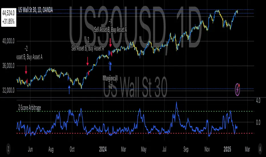
Classic Nacked Z-Score ArbitrageThe “Classic Naked Z-Score Arbitrage” strategy employs a statistical arbitrage model based on the Z-score of the price spread between two assets. This strategy follows the premise of pair trading, where two correlated assets, typically from the same market sector, are traded against each other to profit from relative price movements (Gatev, Goetzmann, & Rouwenhorst, 2006). The approach involves calculating the Z-score of the price spread between two assets to determine market inefficiencies and capitalize on short-term mispricing.
Methodology
Price Spread Calculation:
The strategy calculates the spread between the two selected assets (Asset A and Asset B), typically from different sectors or asset classes, on a daily timeframe.
Statistical Basis – Z-Score:
The Z-score is used as a measure of how far the current price spread deviates from its historical mean, using the standard deviation for normalization.
Trading Logic:
• Long Position:
A long position is initiated when the Z-score exceeds the predefined threshold (e.g., 2.0), indicating that Asset A is undervalued relative to Asset B. This signals an arbitrage opportunity where the trader buys Asset B and sells Asset A.
• Short Position:
A short position is entered when the Z-score falls below the negative threshold, indicating that Asset A is overvalued relative to Asset B. The strategy involves selling Asset B and buying Asset A.
Theoretical Foundation
This strategy is rooted in mean reversion theory, which posits that asset prices tend to return to their long-term average after temporary deviations. This form of arbitrage is widely used in statistical arbitrage and pair trading techniques, where investors seek to exploit short-term price inefficiencies between two assets that historically maintain a stable price relationship (Avery & Sibley, 2020).
Further, the Z-score is an effective tool for identifying significant deviations from the mean, which can be seen as a signal for the potential reversion of the price spread (Braucher, 2015). By capturing these inefficiencies, traders aim to profit from convergence or divergence between correlated assets.
Practical Application
The strategy aligns with the Financial Algorithmic Trading and Market Liquidity analysis, emphasizing the importance of statistical models and efficient execution (Harris, 2024). By utilizing a simple yet effective risk-reward mechanism based on the Z-score, the strategy contributes to the growing body of research on market liquidity, asset correlation, and algorithmic trading.
The integration of transaction costs and slippage ensures that the strategy accounts for practical trading limitations, helping to refine execution in real market conditions. These factors are vital in modern quantitative finance, where liquidity and execution risk can erode profits (Harris, 2024).
References
• Gatev, E., Goetzmann, W. N., & Rouwenhorst, K. G. (2006). Pairs Trading: Performance of a Relative-Value Arbitrage Rule. The Review of Financial Studies, 19(3), 1317-1343.
• Avery, C., & Sibley, D. (2020). Statistical Arbitrage: The Evolution and Practices of Quantitative Trading. Journal of Quantitative Finance, 18(5), 501-523.
• Braucher, J. (2015). Understanding the Z-Score in Trading. Journal of Financial Markets, 12(4), 225-239.
• Harris, L. (2024). Financial Algorithmic Trading and Market Liquidity: A Comprehensive Analysis. Journal of Financial Engineering, 7(1), 18-34.
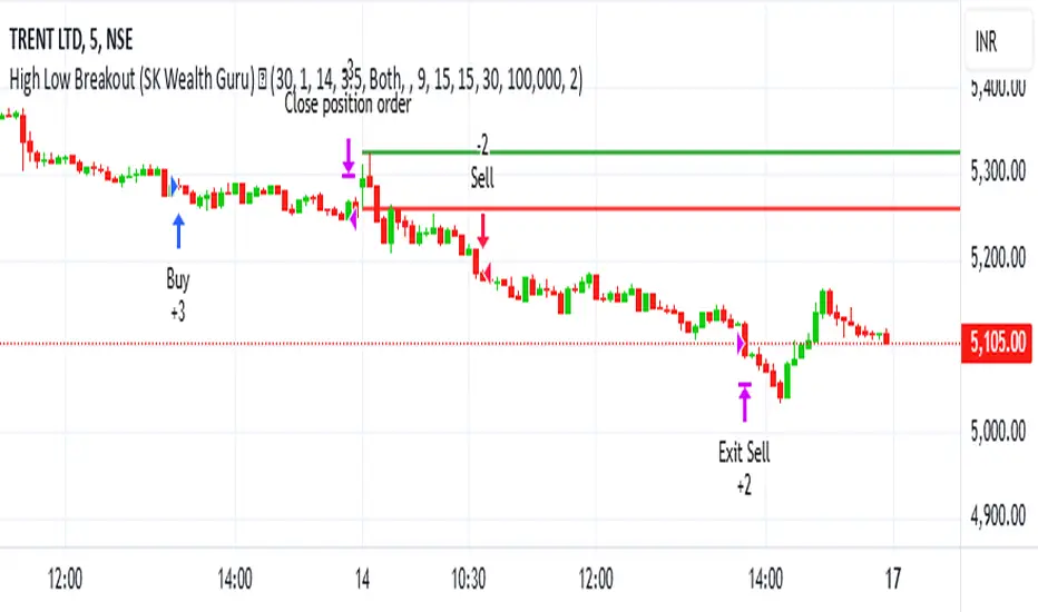
High-Low Breakout Strategy with ATR traling Stop LossThis script is a TradingView Pine Script strategy that implements a High-Low Breakout Strategy with ATR Trailing Stop.created by SK WEALTH GURU, Here’s a breakdown of its key components:
Features and Functionality
Custom Timeframe and High-Low Detection
Allows users to select a custom timeframe (default: 30 minutes) to detect high and low levels.
Tracks the high and low within a user-specified period (e.g., first 30 minutes of the session).
Draws horizontal lines for high and low, persisting for a specified number of days.
Trade Entry Conditions
Long Entry: If the closing price crosses above the recorded high.
Short Entry: If the closing price crosses below the recorded low.
The user can choose to trade Long, Short, or Both.
ATR-Based Trailing Stop & Risk Management
Uses Average True Range (ATR) with a multiplier (default: 3.5) to determine a dynamic trailing stop-loss.
Trades reset daily, ensuring a fresh start each day.
Trade Execution and Partial Profit Taking
Stop-loss: Default at 1% of entry price.
Partial profit: Books 50% of the position at 3% profit.
Max 2 trades per day: If the first trade hits stop-loss, the strategy allows one re-entry.
Intraday Exit Condition
All positions close at 3:15 PM to ensure no overnight risk.
IU Range Trading StrategyIU Range Trading Strategy
The IU Range Trading Strategy is designed to identify range-bound markets and take trades based on defined price ranges. This strategy uses a combination of price ranges and ATR (Average True Range) to filter entry conditions and incorporates a trailing stop-loss mechanism for better trade management.
User Inputs:
- Range Length: Defines the number of bars to calculate the highest and lowest price range (default: 10).
- ATR Length: Sets the length of the ATR calculation (default: 14).
- ATR Stop-Loss Factor: Determines the multiplier for the ATR-based stop-loss (default: 2.00).
Entry Conditions:
1. A range is identified when the difference between the highest and lowest prices over the selected range is less than or equal to 1.75 times the ATR.
2. Once a valid range is formed:
- A long trade is triggered at the range high.
- A short trade is triggered at the range low.
Exit Conditions:
1. Trailing Stop-Loss:
- The stop-loss adjusts dynamically using ATR targets.
- The strategy locks in profits as the trade moves in your favor.
2. The stop-loss and take-profit levels are visually plotted for transparency and easier decision-making.
Features:
- Automated box creation to visualize the trading range.
- Supports one position at a time, canceling opposite-side entries.
- ATR-based trailing stop-loss for effective risk management.
- Clear visual representation of stop-loss and take-profit levels with colored bands.
This strategy works best in markets with defined ranges and can help traders identify breakout opportunities when the price exits the range.

Dynamic Ticks Oscillator Model (DTOM)The Dynamic Ticks Oscillator Model (DTOM) is a systematic trading approach grounded in momentum and volatility analysis, designed to exploit behavioral inefficiencies in the equity markets. It focuses on the NYSE Down Ticks, a metric reflecting the cumulative number of stocks trading at a lower price than their previous trade. As a proxy for market sentiment and selling pressure, this indicator is particularly useful in identifying shifts in investor behavior during periods of heightened uncertainty or volatility (Jegadeesh & Titman, 1993).
Theoretical Basis
The DTOM builds on established principles of momentum and mean reversion in financial markets. Momentum strategies, which seek to capitalize on the persistence of price trends, have been shown to deliver significant returns in various asset classes (Carhart, 1997). However, these strategies are also susceptible to periods of drawdown due to sudden reversals. By incorporating volatility as a dynamic component, DTOM adapts to changing market conditions, addressing one of the primary challenges of traditional momentum models (Barroso & Santa-Clara, 2015).
Sentiment and Volatility as Core Drivers
The NYSE Down Ticks serve as a proxy for short-term negative sentiment. Sudden increases in Down Ticks often signal panic-driven selling, creating potential opportunities for mean reversion. Behavioral finance studies suggest that investor overreaction to negative news can lead to temporary mispricings, which systematic strategies can exploit (De Bondt & Thaler, 1985). By incorporating a rate-of-change (ROC) oscillator into the model, DTOM tracks the momentum of Down Ticks over a specified lookback period, identifying periods of extreme sentiment.
In addition, the strategy dynamically adjusts entry and exit thresholds based on recent volatility. Research indicates that incorporating volatility into momentum strategies can enhance risk-adjusted returns by improving adaptability to market conditions (Moskowitz, Ooi, & Pedersen, 2012). DTOM uses standard deviations of the ROC as a measure of volatility, allowing thresholds to contract during calm markets and expand during turbulent ones. This approach helps mitigate false signals and aligns with findings that volatility scaling can improve strategy robustness (Barroso & Santa-Clara, 2015).
Practical Implications
The DTOM framework is particularly well-suited for systematic traders seeking to exploit behavioral inefficiencies while maintaining adaptability to varying market environments. By leveraging sentiment metrics such as the NYSE Down Ticks and combining them with a volatility-adjusted momentum oscillator, the strategy addresses key limitations of traditional trend-following models, such as their lagging nature and susceptibility to reversals in volatile conditions.
References
• Barroso, P., & Santa-Clara, P. (2015). Momentum Has Its Moments. Journal of Financial Economics, 116(1), 111–120.
• Carhart, M. M. (1997). On Persistence in Mutual Fund Performance. The Journal of Finance, 52(1), 57–82.
• De Bondt, W. F., & Thaler, R. (1985). Does the Stock Market Overreact? The Journal of Finance, 40(3), 793–805.
• Jegadeesh, N., & Titman, S. (1993). Returns to Buying Winners and Selling Losers: Implications for Stock Market Efficiency. The Journal of Finance, 48(1), 65–91.
• Moskowitz, T. J., Ooi, Y. H., & Pedersen, L. H. (2012). Time Series Momentum. Journal of Financial Economics, 104(2), 228–250.

00 Averaging Down Backtest Strategy by RPAlawyer v21FOR EDUCATIONAL PURPOSES ONLY! THE CODE IS NOT YET FULLY DEVELOPED, BUT IT CAN PROVIDE INTERESTING DATA AND INSIGHTS IN ITS CURRENT STATE.
This strategy is an 'averaging down' backtester strategy. The goal of averaging/doubling down is to buy more of an asset at a lower price to reduce your average entry price.
This backtester code proves why you shouldn't do averaging down, but the code can be developed (and will be developed) further, and there might be settings even in its current form that prove that averaging down can be done effectively.
Different averaging down strategies exist:
- Linear/Fixed Amount: buy $1000 every time price drops 5%
- Grid Trading: Placing orders at price levels, often with increasing size, like $1000 at -5%, $2000 at -10%
- Martingale: doubling the position size with each new entry
- Reverse Martingale: decreasing position size as price falls: $4000, then $2000, then $1000
- Percentage-Based: position size based on % of remaining capital, like 10% of available funds at each level
- Dynamic/Adaptive: larger entries during high volatility, smaller during low
- Logarithmic: position sizes increase logarithmically as price drops
Unlike the above average costing strategies, it applies averaging down (I use DCA as a synonym) at a very strong trend reversal. So not at a certain predetermined percentage negative PNL % but at a trend reversal signaled by an indicator - hence it most closely resembles a dynamically moving grid DCA strategy.
Both entering the trade and averaging down assume a strong trend. The signals for trend detection are provided by an indicator that I published under the name '00 Parabolic SAR Trend Following Signals by RPAlawyer', but any indicator that generates numeric signals of 1 and -1 for buy and sell signals can be used.
The indicator must be connected to the strategy: in the strategy settings under 'External Source' you need to select '00 Parabolic SAR Trend Following Signals by RPAlawyer: Connector'. From this point, the strategy detects when the indicator generates buy and sell signals.
The strategy considers a strong trend when a buy signal appears above a very conservative ATR band, or a sell signal below the ATR band. The conservative ATR is chosen to filter ranging markets. This very conservative ATR setting has a default multiplier of 8 and length of 40. The multiplier can be increased up to 10, but there will be very few buy and sell signals at that level and DCA requirements will be very high. Trade entry and DCA occur at these strong trends. In the settings, the 'ATR Filter' setting determines the entry condition (e.g., ATR Filter multiplier of 9), and the 'DCA ATR' determines when DCA will happen (e.g., DCA ATR multiplier of 6).
The DCA levels and DCA amounts are determined as follows:
The first DCA occurs below the DCA Base Deviation% level (see settings, default 3%) which acts as a threshold. The thick green line indicates the long position avg price, and the thin red line below the green line indicates the 3% DCA threshold for long positions. The thick red line indicates the short position avg price, and the thin red line above the thick red line indicates the short position 3% DCA threshold. DCA size multiplier defines the DCA amount invested.
If the loss exceeds 3% AND a buy signal arrives below the lower ATR band for longs, or a sell signal arrives above the upper ATR band for shorts, then the first DCA will be executed. So the first DCA won't happen at 3%, rather 3% is a threshold where the additional condition is that the price must close above or below the ATR band (let's say the first DCA occured at 8%) – this is why the code resembles a dynamic grid strategy, where the grid moves such that alongside the first 3% threshold, a strong trend must also appear for DCA. At this point, the thick green/red line moves because the avg price is modified as a result of the DCA, and the thin red line indicating the next DCA level also moves. The next DCA level is determined by the first DCA level, meaning modified avg price plus an additional +8% + (3% * the Step Scale Multiplier in the settings). This next DCA level will be indicated by the modified thin red line, and the price must break through this level and again break through the ATR band for the second DCA to occur.
Since all this wasn't complicated enough, and I was always obsessed by the idea that when we're sitting in an underwater position for days, doing DCA and waiting for the price to correct, we can actually enter a short position on the other side, on which we can realize profit (if the broker allows taking hedge positions, Binance allows this in Europe).
This opposite position in this strategy can open from the point AFTER THE FIRST DCA OF THE BASE POSITION OCCURS. This base position first DCA actually indicates that the price has already moved against us significantly so time to earn some money on the other side. Breaking through the ATR band is also a condition for entry here, so the hedge position entry is not automatic, and the condition for further DCA is breaking through the DCA Base Deviation (default 3%) and breaking through the ATR band. So for the 'hedge' or rather opposite position, the entry and further DCA conditions are the same as for the base position. The hedge position avg price is indicated by a thick black line and the Next Hedge DCA Level is indicated by a thin black line.
The TPs are indicated by green labels for base positions and red labels for hedge positions.
No SL built into the strategy at this point but you are free to do your coding.
Summary data can be found in the upper right corner.
The fantastic trend reversal indicator Machine learning: Lorentzian Classification by jdehorty can be used as an external indicator, choose 'backtest stream' for the external source. The ATR Band multiplicators need to be reduced to 5-6 when using Lorentz.
The code can be further developed in several aspects, and as I write this, I already have a few ideas 😊

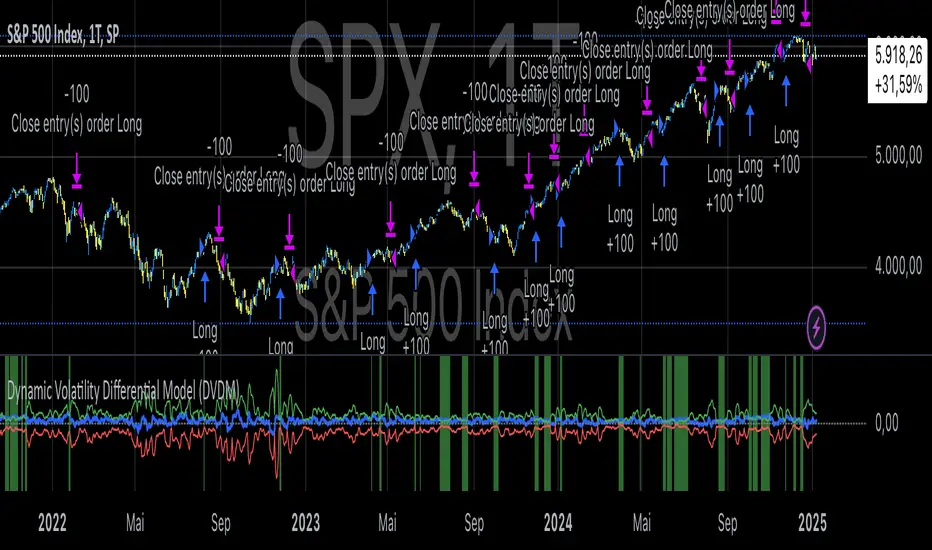
Dynamic Volatility Differential Model (DVDM)The Dynamic Volatility Differential Model (DVDM) is a quantitative trading strategy designed to exploit the spread between implied volatility (IV) and historical (realized) volatility (HV). This strategy identifies trading opportunities by dynamically adjusting thresholds based on the standard deviation of the volatility spread. The DVDM is versatile and applicable across various markets, including equity indices, commodities, and derivatives such as the FDAX (DAX Futures).
Key Components of the DVDM:
1. Implied Volatility (IV):
The IV is derived from options markets and reflects the market’s expectation of future price volatility. For instance, the strategy uses volatility indices such as the VIX (S&P 500), VXN (Nasdaq 100), or RVX (Russell 2000), depending on the target market. These indices serve as proxies for market sentiment and risk perception (Whaley, 2000).
2. Historical Volatility (HV):
The HV is computed from the log returns of the underlying asset’s price. It represents the actual volatility observed in the market over a defined lookback period, adjusted to annualized levels using a multiplier of \sqrt{252} for daily data (Hull, 2012).
3. Volatility Spread:
The difference between IV and HV forms the volatility spread, which is a measure of divergence between market expectations and actual market behavior.
4. Dynamic Thresholds:
Unlike static thresholds, the DVDM employs dynamic thresholds derived from the standard deviation of the volatility spread. The thresholds are scaled by a user-defined multiplier, ensuring adaptability to market conditions and volatility regimes (Christoffersen & Jacobs, 2004).
Trading Logic:
1. Long Entry:
A long position is initiated when the volatility spread exceeds the upper dynamic threshold, signaling that implied volatility is significantly higher than realized volatility. This condition suggests potential mean reversion, as markets may correct inflated risk premiums.
2. Short Entry:
A short position is initiated when the volatility spread falls below the lower dynamic threshold, indicating that implied volatility is significantly undervalued relative to realized volatility. This signals the possibility of increased market uncertainty.
3. Exit Conditions:
Positions are closed when the volatility spread crosses the zero line, signifying a normalization of the divergence.
Advantages of the DVDM:
1. Adaptability:
Dynamic thresholds allow the strategy to adjust to changing market conditions, making it suitable for both low-volatility and high-volatility environments.
2. Quantitative Precision:
The use of standard deviation-based thresholds enhances statistical reliability and reduces subjectivity in decision-making.
3. Market Versatility:
The strategy’s reliance on volatility metrics makes it universally applicable across asset classes and markets, ensuring robust performance.
Scientific Relevance:
The strategy builds on empirical research into the predictive power of implied volatility over realized volatility (Poon & Granger, 2003). By leveraging the divergence between these measures, the DVDM aligns with findings that IV often overestimates future volatility, creating opportunities for mean-reversion trades. Furthermore, the inclusion of dynamic thresholds aligns with risk management best practices by adapting to volatility clustering, a well-documented phenomenon in financial markets (Engle, 1982).
References:
1. Christoffersen, P., & Jacobs, K. (2004). The importance of the volatility risk premium for volatility forecasting. Journal of Financial and Quantitative Analysis, 39(2), 375-397.
2. Engle, R. F. (1982). Autoregressive conditional heteroskedasticity with estimates of the variance of United Kingdom inflation. Econometrica, 50(4), 987-1007.
3. Hull, J. C. (2012). Options, Futures, and Other Derivatives. Pearson Education.
4. Poon, S. H., & Granger, C. W. J. (2003). Forecasting volatility in financial markets: A review. Journal of Economic Literature, 41(2), 478-539.
5. Whaley, R. E. (2000). The investor fear gauge. Journal of Portfolio Management, 26(3), 12-17.
This strategy leverages quantitative techniques and statistical rigor to provide a systematic approach to volatility trading, making it a valuable tool for professional traders and quantitative analysts.