Bollinger Bounce Reversal Strategy – Visual EditionOverview:
The Bollinger Bounce Reversal Strategy – Visual Edition is designed to capture potential reversal moves at price extremes—often termed “bounce points”—by using a combination of technical indicators. The strategy integrates Bollinger Bands, MACD, and volume analysis, and it provides rich on‑chart visual cues to help traders understand its signals and conditions. Additionally, the strategy enforces a maximum of 5 trades per day and uses fixed risk management parameters. This publication is intended for educational purposes and offers a systematic, transparent approach that you can further adjust to fit your market or risk profile.
How It Works:
Bollinger Bands:
A 20‑period simple moving average (SMA) and a user‑defined standard deviation multiplier (default 2.0) are used to calculate the Bollinger Bands.
When the price reaches or crosses these bands (i.e. falls below the lower band or rises above the upper band), it suggests that the price is in an extreme, potentially oversold or overbought, state.
MACD Filter:
The MACD (calculated with standard lengths, e.g. 12, 26, 9) provides momentum information.
For a bullish (long) signal, the MACD line should be above its signal line; for a bearish (short) signal, the MACD line should be below.
Volume Confirmation:
The strategy uses a 20‑period volume moving average to determine if current volume is strong enough to validate a signal.
A signal is confirmed only if the current volume is at or above a specified multiple (by default, 1.0×) of this moving average, ensuring that the move is supported by increased market participation.
Visual Cues:
Bollinger Bands and Fill: The basis (SMA), upper, and lower Bollinger Bands are plotted, and the area between the upper and lower bands is filled with a semi‑transparent color.
Signal Markers: When a long or short signal is generated, corresponding markers (labels) appear on the chart.
Background Coloring: The chart’s background changes color (green for long signals and red for short signals) on the bars where signals occur.
Information Table: An on‑chart table displays key indicator values (MACD, signal line, volume, average volume) and the number of trades executed that day.
Entry Conditions:
Long Entry:
A long trade is triggered when the previous bar’s close is below the lower Bollinger Band and the current bar’s close crosses above it, combined with a bullish MACD condition and strong volume.
Short Entry:
A short trade is triggered when the previous bar’s close is above the upper Bollinger Band and the current bar’s close crosses below it, with a bearish MACD condition and high volume.
Risk Management:
Daily Trade Limit: The strategy restricts trading to no more than 5 trades per day.
Stop-Loss and Take-Profit:
For each position, a stop loss is set at a fixed percentage away from the entry price (typically 2%), and a take profit is set to target a 1:2 risk-reward ratio (typically 4% from the entry price).
Backtesting Setup:
Initial Capital: $10,000
Commission: 0.1% per trade
Slippage: 1 tick per bar
These realistic parameters help ensure that backtesting results reflect the conditions of an average trader.
Disclaimer:
Past performance is not indicative of future results. This strategy is experimental and provided solely for educational purposes. It is essential to backtest extensively and paper trade before any live deployment. All risk management practices are advisory, and you should adjust parameters to suit your own trading style and risk tolerance.
Conclusion:
By combining Bollinger Bands, MACD, and volume analysis, the Bollinger Bounce Reversal Strategy – Visual Edition provides a clear, systematic method to identify potential reversal opportunities at price extremes. The added visual cues help traders quickly interpret signals and assess market conditions, while strict risk management and a daily trade cap help keep trading disciplined. Adjust and refine the settings as needed to better suit your specific market and risk profile.
Volatility

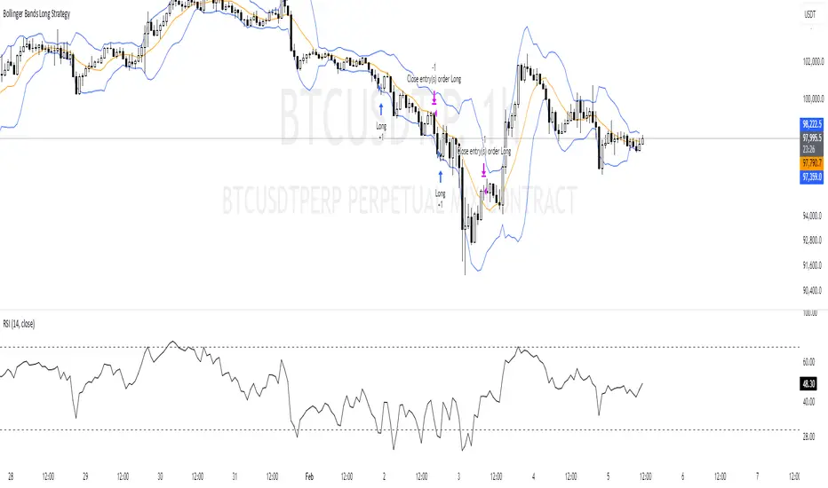
Bollinger Bands Long Strategy
This strategy is designed for identifying and executing long trades based on Bollinger Bands and RSI. It aims to capitalize on potential oversold conditions and subsequent price recovery.
Key Features:
- Bollinger Bands (10,2): The strategy uses Bollinger Bands with a 10-period moving average and a multiplier of 2 to define price volatility.
- RSI Filter: A trade is only triggered when the RSI (14-period) is below 30, ensuring entry during oversold conditions.
- Entry Condition: A long trade is entered immediately when the price crosses below the lower Bollinger Band and the RSI is under 30.
- Exit Condition: The position is exited when the price reaches or crosses above the Bollinger Band basis (20-period moving average).
Best Used For:
- Identifying oversold conditions with a strong potential for a rebound.
- Markets or assets with clear oscillations and volatility e.g., BTC.
**Disclaimer:** This strategy is for educational purposes and should be used with caution. Backtesting and risk management are essential before live trading.
GOLD Volume-Based Entry StrategyShort Description:
This script identifies potential long entries by detecting two consecutive bars with above-average volume and bullish price action. When these conditions are met, a trade is entered, and an optional profit target is set based on user input. This strategy can help highlight momentum-driven breakouts or trend continuations triggered by a surge in buying volume.
How It Works
Volume Moving Average
A simple moving average of volume (vol_ma) is calculated over a user-defined period (default: 20 bars). This helps us distinguish when volume is above or below recent averages.
Consecutive Green Volume Bars
First bar: Must be bullish (close > open) and have volume above the volume MA.
Second bar: Must also be bullish, with volume above the volume MA and higher than the first bar’s volume.
When these two bars appear in sequence, we interpret it as strong buying pressure that could drive price higher.
Entry & Profit Target
Upon detecting these two consecutive bullish bars, the script places a long entry.
A profit target is set at current price plus a user-defined fixed amount (default: 5 USD).
You can adjust this target, or you can add a stop-loss in the script to manage risk further.
Visual Cues
Buy Signal Marker appears on the chart when the second bar confirms the signal.
Green Volume Columns highlight the bars that fulfill the criteria, providing a quick visual confirmation of high-volume bullish bars.
Works fine on 1M-2M-5M-15M-30M. Do not use it on higher TF. Due the lack of historical data on lower TF, the backtest result is limited.

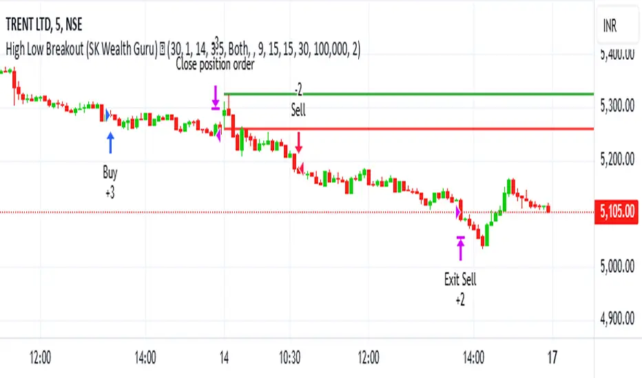
High-Low Breakout Strategy with ATR traling Stop LossThis script is a TradingView Pine Script strategy that implements a High-Low Breakout Strategy with ATR Trailing Stop.created by SK WEALTH GURU, Here’s a breakdown of its key components:
Features and Functionality
Custom Timeframe and High-Low Detection
Allows users to select a custom timeframe (default: 30 minutes) to detect high and low levels.
Tracks the high and low within a user-specified period (e.g., first 30 minutes of the session).
Draws horizontal lines for high and low, persisting for a specified number of days.
Trade Entry Conditions
Long Entry: If the closing price crosses above the recorded high.
Short Entry: If the closing price crosses below the recorded low.
The user can choose to trade Long, Short, or Both.
ATR-Based Trailing Stop & Risk Management
Uses Average True Range (ATR) with a multiplier (default: 3.5) to determine a dynamic trailing stop-loss.
Trades reset daily, ensuring a fresh start each day.
Trade Execution and Partial Profit Taking
Stop-loss: Default at 1% of entry price.
Partial profit: Books 50% of the position at 3% profit.
Max 2 trades per day: If the first trade hits stop-loss, the strategy allows one re-entry.
Intraday Exit Condition
All positions close at 3:15 PM to ensure no overnight risk.
IU Range Trading StrategyIU Range Trading Strategy
The IU Range Trading Strategy is designed to identify range-bound markets and take trades based on defined price ranges. This strategy uses a combination of price ranges and ATR (Average True Range) to filter entry conditions and incorporates a trailing stop-loss mechanism for better trade management.
User Inputs:
- Range Length: Defines the number of bars to calculate the highest and lowest price range (default: 10).
- ATR Length: Sets the length of the ATR calculation (default: 14).
- ATR Stop-Loss Factor: Determines the multiplier for the ATR-based stop-loss (default: 2.00).
Entry Conditions:
1. A range is identified when the difference between the highest and lowest prices over the selected range is less than or equal to 1.75 times the ATR.
2. Once a valid range is formed:
- A long trade is triggered at the range high.
- A short trade is triggered at the range low.
Exit Conditions:
1. Trailing Stop-Loss:
- The stop-loss adjusts dynamically using ATR targets.
- The strategy locks in profits as the trade moves in your favor.
2. The stop-loss and take-profit levels are visually plotted for transparency and easier decision-making.
Features:
- Automated box creation to visualize the trading range.
- Supports one position at a time, canceling opposite-side entries.
- ATR-based trailing stop-loss for effective risk management.
- Clear visual representation of stop-loss and take-profit levels with colored bands.
This strategy works best in markets with defined ranges and can help traders identify breakout opportunities when the price exits the range.

Dynamic Ticks Oscillator Model (DTOM)The Dynamic Ticks Oscillator Model (DTOM) is a systematic trading approach grounded in momentum and volatility analysis, designed to exploit behavioral inefficiencies in the equity markets. It focuses on the NYSE Down Ticks, a metric reflecting the cumulative number of stocks trading at a lower price than their previous trade. As a proxy for market sentiment and selling pressure, this indicator is particularly useful in identifying shifts in investor behavior during periods of heightened uncertainty or volatility (Jegadeesh & Titman, 1993).
Theoretical Basis
The DTOM builds on established principles of momentum and mean reversion in financial markets. Momentum strategies, which seek to capitalize on the persistence of price trends, have been shown to deliver significant returns in various asset classes (Carhart, 1997). However, these strategies are also susceptible to periods of drawdown due to sudden reversals. By incorporating volatility as a dynamic component, DTOM adapts to changing market conditions, addressing one of the primary challenges of traditional momentum models (Barroso & Santa-Clara, 2015).
Sentiment and Volatility as Core Drivers
The NYSE Down Ticks serve as a proxy for short-term negative sentiment. Sudden increases in Down Ticks often signal panic-driven selling, creating potential opportunities for mean reversion. Behavioral finance studies suggest that investor overreaction to negative news can lead to temporary mispricings, which systematic strategies can exploit (De Bondt & Thaler, 1985). By incorporating a rate-of-change (ROC) oscillator into the model, DTOM tracks the momentum of Down Ticks over a specified lookback period, identifying periods of extreme sentiment.
In addition, the strategy dynamically adjusts entry and exit thresholds based on recent volatility. Research indicates that incorporating volatility into momentum strategies can enhance risk-adjusted returns by improving adaptability to market conditions (Moskowitz, Ooi, & Pedersen, 2012). DTOM uses standard deviations of the ROC as a measure of volatility, allowing thresholds to contract during calm markets and expand during turbulent ones. This approach helps mitigate false signals and aligns with findings that volatility scaling can improve strategy robustness (Barroso & Santa-Clara, 2015).
Practical Implications
The DTOM framework is particularly well-suited for systematic traders seeking to exploit behavioral inefficiencies while maintaining adaptability to varying market environments. By leveraging sentiment metrics such as the NYSE Down Ticks and combining them with a volatility-adjusted momentum oscillator, the strategy addresses key limitations of traditional trend-following models, such as their lagging nature and susceptibility to reversals in volatile conditions.
References
• Barroso, P., & Santa-Clara, P. (2015). Momentum Has Its Moments. Journal of Financial Economics, 116(1), 111–120.
• Carhart, M. M. (1997). On Persistence in Mutual Fund Performance. The Journal of Finance, 52(1), 57–82.
• De Bondt, W. F., & Thaler, R. (1985). Does the Stock Market Overreact? The Journal of Finance, 40(3), 793–805.
• Jegadeesh, N., & Titman, S. (1993). Returns to Buying Winners and Selling Losers: Implications for Stock Market Efficiency. The Journal of Finance, 48(1), 65–91.
• Moskowitz, T. J., Ooi, Y. H., & Pedersen, L. H. (2012). Time Series Momentum. Journal of Financial Economics, 104(2), 228–250.

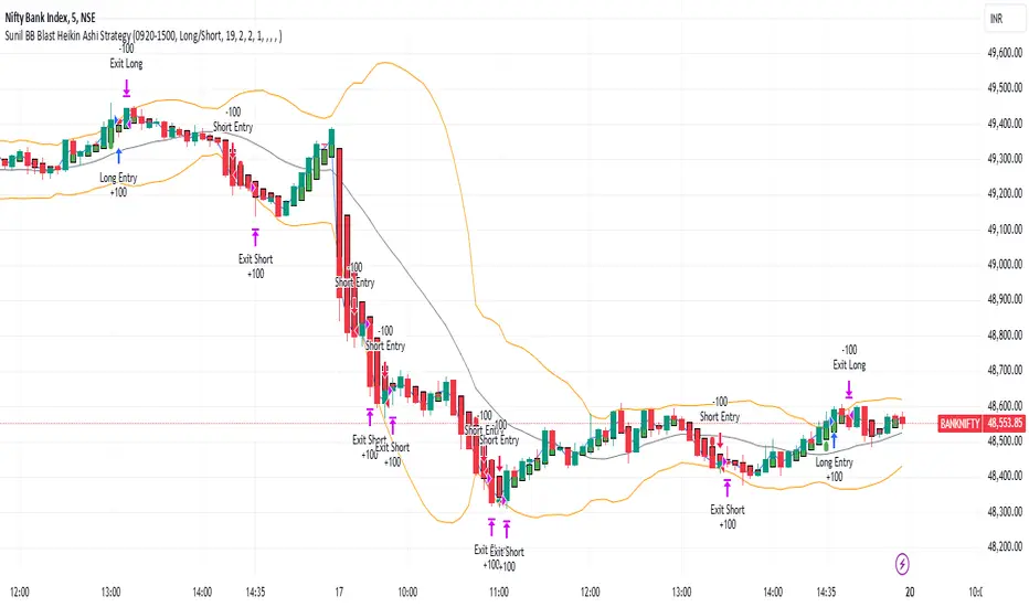
Sunil BB Blast Heikin Ashi StrategySunil BB Blast Heikin Ashi Strategy
The Sunil BB Blast Heikin Ashi Strategy is a trend-following trading strategy that combines Bollinger Bands with Heikin-Ashi candles for precise market entries and exits. It aims to capitalize on price volatility while ensuring controlled risk through dynamic stop-loss and take-profit levels based on a user-defined Risk-to-Reward Ratio (RRR).
Key Features:
Trading Window:
The strategy operates within a user-defined time window (e.g., from 09:20 to 15:00) to align with market hours or other preferred trading sessions.
Trade Direction:
Users can select between Long Only, Short Only, or Long/Short trade directions, allowing flexibility depending on market conditions.
Bollinger Bands:
Bollinger Bands are used to identify potential breakout or breakdown zones. The strategy enters trades when price breaks through the upper or lower Bollinger Band, indicating a possible trend continuation.
Heikin-Ashi Candles:
Heikin-Ashi candles help smooth price action and filter out market noise. The strategy uses these candles to confirm trend direction and improve entry accuracy.
Risk Management (Risk-to-Reward Ratio):
The strategy automatically adjusts the take-profit (TP) level and stop-loss (SL) based on the selected Risk-to-Reward Ratio (RRR). This ensures that trades are risk-managed effectively.
Automated Alerts and Webhooks:
The strategy includes automated alerts for trade entries and exits. Users can set up JSON webhooks for external execution or trading automation.
Active Position Tracking:
The strategy tracks whether there is an active position (long or short) and only exits when price hits the pre-defined SL or TP levels.
Exit Conditions:
The strategy exits positions when either the take-profit (TP) or stop-loss (SL) levels are hit, ensuring risk management is adhered to.
Default Settings:
Trading Window:
09:20-15:00
This setting confines the strategy to the specified hours, ensuring trading only occurs during active market hours.
Strategy Direction:
Default: Long/Short
This allows for both long and short trades depending on market conditions. You can select "Long Only" or "Short Only" if you prefer to trade in one direction.
Bollinger Band Length (bbLength):
Default: 19
Length of the moving average used to calculate the Bollinger Bands.
Bollinger Band Multiplier (bbMultiplier):
Default: 2.0
Multiplier used to calculate the upper and lower bands. A higher multiplier increases the width of the bands, leading to fewer but more significant trades.
Take Profit Multiplier (tpMultiplier):
Default: 2.0
Multiplier used to determine the take-profit level based on the calculated stop-loss. This ensures that the profit target aligns with the selected Risk-to-Reward Ratio.
Risk-to-Reward Ratio (RRR):
Default: 1.0
The ratio used to calculate the take-profit relative to the stop-loss. A higher RRR means larger profit targets.
Trade Automation (JSON Webhooks):
Allows for integration with external systems for automated execution:
Long Entry JSON: Customizable entry condition for long positions.
Long Exit JSON: Customizable exit condition for long positions.
Short Entry JSON: Customizable entry condition for short positions.
Short Exit JSON: Customizable exit condition for short positions.
Entry Logic:
Long Entry:
The strategy enters a long position when:
The Heikin-Ashi candle shows a bullish trend (green close > open).
The price is above the upper Bollinger Band, signaling a breakout.
The previous candle also closed higher than it opened.
Short Entry:
The strategy enters a short position when:
The Heikin-Ashi candle shows a bearish trend (red close < open).
The price is below the lower Bollinger Band, signaling a breakdown.
The previous candle also closed lower than it opened.
Exit Logic:
Take-Profit (TP):
The take-profit level is calculated as a multiple of the distance between the entry price and the stop-loss level, determined by the selected Risk-to-Reward Ratio (RRR).
Stop-Loss (SL):
The stop-loss is placed at the opposite Bollinger Band level (lower for long positions, upper for short positions).
Exit Trigger:
The strategy exits a trade when either the take-profit or stop-loss level is hit.
Plotting and Visuals:
The Heikin-Ashi candles are displayed on the chart, with green candles for uptrends and red candles for downtrends.
Bollinger Bands (upper, lower, and basis) are plotted for visual reference.
Entry points for long and short trades are marked with green and red labels below and above bars, respectively.
Strategy Alerts:
Alerts are triggered when:
A long entry condition is met.
A short entry condition is met.
A trade exits (either via take-profit or stop-loss).
These alerts can be used to trigger notifications or webhook events for automated trading systems.
Notes:
The strategy is designed for use on intraday charts but can be applied to any timeframe.
It is highly customizable, allowing for tailored risk management and trading windows.
The Sunil BB Blast Heikin Ashi Strategy combines two powerful technical analysis tools (Bollinger Bands and Heikin-Ashi candles) with strong risk management, making it suitable for both beginners and experienced traders.
Feebacks are welcome from the users.
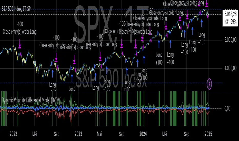
Dynamic Volatility Differential Model (DVDM)The Dynamic Volatility Differential Model (DVDM) is a quantitative trading strategy designed to exploit the spread between implied volatility (IV) and historical (realized) volatility (HV). This strategy identifies trading opportunities by dynamically adjusting thresholds based on the standard deviation of the volatility spread. The DVDM is versatile and applicable across various markets, including equity indices, commodities, and derivatives such as the FDAX (DAX Futures).
Key Components of the DVDM:
1. Implied Volatility (IV):
The IV is derived from options markets and reflects the market’s expectation of future price volatility. For instance, the strategy uses volatility indices such as the VIX (S&P 500), VXN (Nasdaq 100), or RVX (Russell 2000), depending on the target market. These indices serve as proxies for market sentiment and risk perception (Whaley, 2000).
2. Historical Volatility (HV):
The HV is computed from the log returns of the underlying asset’s price. It represents the actual volatility observed in the market over a defined lookback period, adjusted to annualized levels using a multiplier of \sqrt{252} for daily data (Hull, 2012).
3. Volatility Spread:
The difference between IV and HV forms the volatility spread, which is a measure of divergence between market expectations and actual market behavior.
4. Dynamic Thresholds:
Unlike static thresholds, the DVDM employs dynamic thresholds derived from the standard deviation of the volatility spread. The thresholds are scaled by a user-defined multiplier, ensuring adaptability to market conditions and volatility regimes (Christoffersen & Jacobs, 2004).
Trading Logic:
1. Long Entry:
A long position is initiated when the volatility spread exceeds the upper dynamic threshold, signaling that implied volatility is significantly higher than realized volatility. This condition suggests potential mean reversion, as markets may correct inflated risk premiums.
2. Short Entry:
A short position is initiated when the volatility spread falls below the lower dynamic threshold, indicating that implied volatility is significantly undervalued relative to realized volatility. This signals the possibility of increased market uncertainty.
3. Exit Conditions:
Positions are closed when the volatility spread crosses the zero line, signifying a normalization of the divergence.
Advantages of the DVDM:
1. Adaptability:
Dynamic thresholds allow the strategy to adjust to changing market conditions, making it suitable for both low-volatility and high-volatility environments.
2. Quantitative Precision:
The use of standard deviation-based thresholds enhances statistical reliability and reduces subjectivity in decision-making.
3. Market Versatility:
The strategy’s reliance on volatility metrics makes it universally applicable across asset classes and markets, ensuring robust performance.
Scientific Relevance:
The strategy builds on empirical research into the predictive power of implied volatility over realized volatility (Poon & Granger, 2003). By leveraging the divergence between these measures, the DVDM aligns with findings that IV often overestimates future volatility, creating opportunities for mean-reversion trades. Furthermore, the inclusion of dynamic thresholds aligns with risk management best practices by adapting to volatility clustering, a well-documented phenomenon in financial markets (Engle, 1982).
References:
1. Christoffersen, P., & Jacobs, K. (2004). The importance of the volatility risk premium for volatility forecasting. Journal of Financial and Quantitative Analysis, 39(2), 375-397.
2. Engle, R. F. (1982). Autoregressive conditional heteroskedasticity with estimates of the variance of United Kingdom inflation. Econometrica, 50(4), 987-1007.
3. Hull, J. C. (2012). Options, Futures, and Other Derivatives. Pearson Education.
4. Poon, S. H., & Granger, C. W. J. (2003). Forecasting volatility in financial markets: A review. Journal of Economic Literature, 41(2), 478-539.
5. Whaley, R. E. (2000). The investor fear gauge. Journal of Portfolio Management, 26(3), 12-17.
This strategy leverages quantitative techniques and statistical rigor to provide a systematic approach to volatility trading, making it a valuable tool for professional traders and quantitative analysts.
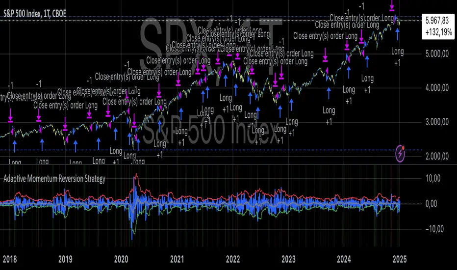
Adaptive Momentum Reversion StrategyThe Adaptive Momentum Reversion Strategy: An Empirical Approach to Market Behavior
The Adaptive Momentum Reversion Strategy seeks to capitalize on market price dynamics by combining concepts from momentum and mean reversion theories. This hybrid approach leverages a Rate of Change (ROC) indicator along with Bollinger Bands to identify overbought and oversold conditions, triggering trades based on the crossing of specific thresholds. The strategy aims to detect momentum shifts and exploit price reversions to their mean.
Theoretical Framework
Momentum and Mean Reversion: Momentum trading assumes that assets with a recent history of strong performance will continue in that direction, while mean reversion suggests that assets tend to return to their historical average over time (Fama & French, 1988; Poterba & Summers, 1988). This strategy incorporates elements of both, looking for periods when momentum is either overextended (and likely to revert) or when the asset’s price is temporarily underpriced relative to its historical trend.
Rate of Change (ROC): The ROC is a straightforward momentum indicator that measures the percentage change in price over a specified period (Wilder, 1978). The strategy calculates the ROC over a 2-period window, making it responsive to short-term price changes. By using ROC, the strategy aims to detect price acceleration and deceleration.
Bollinger Bands: Bollinger Bands are used to identify volatility and potential price extremes, often signaling overbought or oversold conditions. The bands consist of a moving average and two standard deviation bounds that adjust dynamically with price volatility (Bollinger, 2002).
The strategy employs two sets of Bollinger Bands: one for short-term volatility (lower band) and another for longer-term trends (upper band), with different lengths and standard deviation multipliers.
Strategy Construction
Indicator Inputs:
ROC Period: The rate of change is computed over a 2-period window, which provides sensitivity to short-term price fluctuations.
Bollinger Bands:
Lower Band: Calculated with a 18-period length and a standard deviation of 1.7.
Upper Band: Calculated with a 21-period length and a standard deviation of 2.1.
Calculations:
ROC Calculation: The ROC is computed by comparing the current close price to the close price from rocPeriod days ago, expressing it as a percentage.
Bollinger Bands: The strategy calculates both upper and lower Bollinger Bands around the ROC, using a simple moving average as the central basis. The lower Bollinger Band is used as a reference for identifying potential long entry points when the ROC crosses above it, while the upper Bollinger Band serves as a reference for exits, when the ROC crosses below it.
Trading Conditions:
Long Entry: A long position is initiated when the ROC crosses above the lower Bollinger Band, signaling a potential shift from a period of low momentum to an increase in price movement.
Exit Condition: A position is closed when the ROC crosses under the upper Bollinger Band, or when the ROC drops below the lower band again, indicating a reversal or weakening of momentum.
Visual Indicators:
ROC Plot: The ROC is plotted as a line to visualize the momentum direction.
Bollinger Bands: The upper and lower bands, along with their basis (simple moving averages), are plotted to delineate the expected range for the ROC.
Background Color: To enhance decision-making, the strategy colors the background when extreme conditions are detected—green for oversold (ROC below the lower band) and red for overbought (ROC above the upper band), indicating potential reversal zones.
Strategy Performance Considerations
The use of Bollinger Bands in this strategy provides an adaptive framework that adjusts to changing market volatility. When volatility increases, the bands widen, allowing for larger price movements, while during quieter periods, the bands contract, reducing trade signals. This adaptiveness is critical in maintaining strategy effectiveness across different market conditions.
The strategy’s pyramiding setting is disabled (pyramiding=0), ensuring that only one position is taken at a time, which is a conservative risk management approach. Additionally, the strategy includes transaction costs and slippage parameters to account for real-world trading conditions.
Empirical Evidence and Relevance
The combination of momentum and mean reversion has been widely studied and shown to provide profitable opportunities under certain market conditions. Studies such as Jegadeesh and Titman (1993) confirm that momentum strategies tend to work well in trending markets, while mean reversion strategies have been effective during periods of high volatility or after sharp price movements (De Bondt & Thaler, 1985). By integrating both strategies into one system, the Adaptive Momentum Reversion Strategy may be able to capitalize on both trending and reverting market behavior.
Furthermore, research by Chan (1996) on momentum-based trading systems demonstrates that adaptive strategies, which adjust to changes in market volatility, often outperform static strategies, providing a compelling rationale for the use of Bollinger Bands in this context.
Conclusion
The Adaptive Momentum Reversion Strategy provides a robust framework for trading based on the dual concepts of momentum and mean reversion. By using ROC in combination with Bollinger Bands, the strategy is capable of identifying overbought and oversold conditions while adapting to changing market conditions. The use of adaptive indicators ensures that the strategy remains flexible and can perform across different market environments, potentially offering a competitive edge for traders who seek to balance risk and reward in their trading approaches.
References
Bollinger, J. (2002). Bollinger on Bollinger Bands. McGraw-Hill Professional.
Chan, L. K. C. (1996). Momentum, Mean Reversion, and the Cross-Section of Stock Returns. Journal of Finance, 51(5), 1681-1713.
De Bondt, W. F., & Thaler, R. H. (1985). Does the Stock Market Overreact? Journal of Finance, 40(3), 793-805.
Fama, E. F., & French, K. R. (1988). Permanent and Temporary Components of Stock Prices. Journal of Political Economy, 96(2), 246-273.
Jegadeesh, N., & Titman, S. (1993). Returns to Buying Winners and Selling Losers: Implications for Stock Market Efficiency. Journal of Finance, 48(1), 65-91.
Poterba, J. M., & Summers, L. H. (1988). Mean Reversion in Stock Prices: Evidence and Implications. Journal of Financial Economics, 22(1), 27-59.
Wilder, J. W. (1978). New Concepts in Technical Trading Systems. Trend Research.
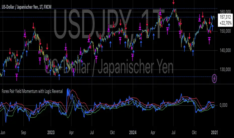
Forex Pair Yield Momentum This Pine Script strategy leverages yield differentials between the 2-year government bond yields of two countries to trade Forex pairs. Yield spreads are widely regarded as a fundamental driver of currency movements, as highlighted by international finance theories like the Interest Rate Parity (IRP), which suggests that currencies with higher yields tend to appreciate due to increased capital flows:
1. Dynamic Yield Spread Calculation:
• The strategy dynamically calculates the yield spread (yield_a - yield_b) for the chosen Forex pair.
• Example: For GBP/USD, the spread equals US 2Y Yield - UK 2Y Yield.
2. Momentum Analysis via Bollinger Bands:
• Yield momentum is computed as the difference between the current spread and its moving
Bollinger Bands are applied to identify extreme deviations:
• Long Entry: When momentum crosses below the lower band.
• Short Entry: When momentum crosses above the upper band.
3. Reversal Logic:
• An optional checkbox reverses the trading logic, allowing long trades at the upper band and short trades at the lower band, accommodating different market conditions.
4. Trade Management:
• Positions are held for a predefined number of bars (hold_periods), and each trade uses a fixed contract size of 100 with a starting capital of $20,000.
Theoretical Basis:
1. Yield Differentials and Currency Movements:
• Empirical studies, such as Clarida et al. (2009), confirm that interest rate differentials significantly impact exchange rate dynamics, especially in carry trade strategies .
• Higher-yields tend to appreciate against lower-yielding currencies due to speculative flows and demand for higher returns.
2. Bollinger Bands for Momentum:
• Bollinger Bands effectively capture deviations in yield momentum, identifying opportunities where price returns to equilibrium (mean reversion) or extends in trend-following scenarios (momentum breakout).
• As Bollinger (2001) emphasized, this tool adapts to market volatility by dynamically adjusting thresholds .
References:
1. Dornbusch, R. (1976). Expectations and Exchange Rate Dynamics. Journal of Political Economy.
2. Obstfeld, M., & Rogoff, K. (1996). Foundations of International Macroeconomics.
3. Clarida, R., Davis, J., & Pedersen, N. (2009). Currency Carry Trade Regimes. NBER.
4. Bollinger, J. (2001). Bollinger on Bollinger Bands.
5. Mendelsohn, L. B. (2006). Forex Trading Using Intermarket Analysis.
Kernel Regression Envelope with SMI OscillatorThis script combines the predictive capabilities of the **Nadaraya-Watson estimator**, implemented by the esteemed jdehorty (credit to him for his excellent work on the `KernelFunctions` library and the original Nadaraya-Watson Envelope indicator), with the confirmation strength of the **Stochastic Momentum Index (SMI)** to create a dynamic trend reversal strategy. The core idea is to identify potential overbought and oversold conditions using the Nadaraya-Watson Envelope and then confirm these signals with the SMI before entering a trade.
**Understanding the Nadaraya-Watson Envelope:**
The Nadaraya-Watson estimator is a non-parametric regression technique that essentially calculates a weighted average of past price data to estimate the current underlying trend. Unlike simple moving averages that give equal weight to all past data within a defined period, the Nadaraya-Watson estimator uses a **kernel function** (in this case, the Rational Quadratic Kernel) to assign weights. The key parameters influencing this estimation are:
* **Lookback Window (h):** This determines how many historical bars are considered for the estimation. A larger window results in a smoother estimation, while a smaller window makes it more reactive to recent price changes.
* **Relative Weighting (alpha):** This parameter controls the influence of different time frames in the estimation. Lower values emphasize longer-term price action, while higher values make the estimator more sensitive to shorter-term movements.
* **Start Regression at Bar (x\_0):** This allows you to exclude the potentially volatile initial bars of a chart from the calculation, leading to a more stable estimation.
The script calculates the Nadaraya-Watson estimation for the closing price (`yhat_close`), as well as the highs (`yhat_high`) and lows (`yhat_low`). The `yhat_close` is then used as the central trend line.
**Dynamic Envelope Bands with ATR:**
To identify potential entry and exit points around the Nadaraya-Watson estimation, the script uses **Average True Range (ATR)** to create dynamic envelope bands. ATR measures the volatility of the price. By multiplying the ATR by different factors (`nearFactor` and `farFactor`), we create multiple bands:
* **Near Bands:** These are closer to the Nadaraya-Watson estimation and are intended to identify potential immediate overbought or oversold zones.
* **Far Bands:** These are further away and can act as potential take-profit or stop-loss levels, representing more extreme price extensions.
The script calculates both near and far upper and lower bands, as well as an average between the near and far bands. This provides a nuanced view of potential support and resistance levels around the estimated trend.
**Confirming Reversals with the Stochastic Momentum Index (SMI):**
While the Nadaraya-Watson Envelope identifies potential overextended conditions, the **Stochastic Momentum Index (SMI)** is used to confirm a potential trend reversal. The SMI, unlike a traditional stochastic oscillator, oscillates around a zero line. It measures the location of the current closing price relative to the median of the high/low range over a specified period.
The script calculates the SMI on a **higher timeframe** (defined by the "Timeframe" input) to gain a broader perspective on the market momentum. This helps to filter out potential whipsaws and false signals that might occur on the current chart's timeframe. The SMI calculation involves:
* **%K Length:** The lookback period for calculating the highest high and lowest low.
* **%D Length:** The period for smoothing the relative range.
* **EMA Length:** The period for smoothing the SMI itself.
The script uses a double EMA for smoothing within the SMI calculation for added smoothness.
**How the Indicators Work Together in the Strategy:**
The strategy enters a long position when:
1. The closing price crosses below the **near lower band** of the Nadaraya-Watson Envelope, suggesting a potential oversold condition.
2. The SMI crosses above its EMA, indicating positive momentum.
3. The SMI value is below -50, further supporting the oversold idea on the higher timeframe.
Conversely, the strategy enters a short position when:
1. The closing price crosses above the **near upper band** of the Nadaraya-Watson Envelope, suggesting a potential overbought condition.
2. The SMI crosses below its EMA, indicating negative momentum.
3. The SMI value is above 50, further supporting the overbought idea on the higher timeframe.
Trades are closed when the price crosses the **far band** in the opposite direction of the trade. A stop-loss is also implemented based on a fixed value.
**In essence:** The Nadaraya-Watson Envelope identifies areas where the price might be deviating significantly from its estimated trend. The SMI, calculated on a higher timeframe, then acts as a confirmation signal, suggesting that the momentum is shifting in the direction of a potential reversal. The ATR-based bands provide dynamic entry and exit points based on the current volatility.
**How to Use the Script:**
1. **Apply the script to your chart.**
2. **Adjust the "Kernel Settings":**
* **Lookback Window (h):** Experiment with different values to find the smoothness that best suits the asset and timeframe you are trading. Lower values make the envelope more reactive, while higher values make it smoother.
* **Relative Weighting (alpha):** Adjust to control the influence of different timeframes on the Nadaraya-Watson estimation.
* **Start Regression at Bar (x\_0):** Increase this value if you want to exclude the initial, potentially volatile, bars from the calculation.
* **Stoploss:** Set your desired stop-loss value.
3. **Adjust the "SMI" settings:**
* **%K Length, %D Length, EMA Length:** These parameters control the sensitivity and smoothness of the SMI. Experiment to find settings that work well for your trading style.
* **Timeframe:** Select the higher timeframe you want to use for SMI confirmation.
4. **Adjust the "ATR Length" and "Near/Far ATR Factor":** These settings control the width and sensitivity of the envelope bands. Smaller ATR lengths make the bands more reactive to recent volatility.
5. **Customize the "Color Settings"** to your preference.
6. **Observe the plots:**
* The **Nadaraya-Watson Estimation (yhat)** line represents the estimated underlying trend.
* The **near and far upper and lower bands** visualize potential overbought and oversold zones based on the ATR.
* The **fill areas** highlight the regions between the near and far bands.
7. **Look for entry signals:** A long entry is considered when the price touches or crosses below the lower near band and the SMI confirms upward momentum. A short entry is considered when the price touches or crosses above the upper near band and the SMI confirms downward momentum.
8. **Manage your trades:** The script provides exit signals when the price crosses the far band. The fixed stop-loss will also close trades if the price moves against your position.
**Justification for Combining Nadaraya-Watson Envelope and SMI:**
The combination of the Nadaraya-Watson Envelope and the SMI provides a more robust approach to identifying potential trend reversals compared to using either indicator in isolation. The Nadaraya-Watson Envelope excels at identifying potential areas where the price is overextended relative to its recent history. However, relying solely on the envelope can lead to false signals, especially in choppy or volatile markets. By incorporating the SMI as a confirmation tool, we add a momentum filter that helps to validate the potential reversals signaled by the envelope. The higher timeframe SMI further helps to filter out noise and focus on more significant shifts in momentum. The ATR-based bands add a dynamic element to the entry and exit points, adapting to the current market volatility. This mashup aims to leverage the strengths of each indicator to create a more reliable trading strategy.

Z-Strike RecoveryThis strategy utilizes the Z-Score of daily changes in the VIX (Volatility Index) to identify moments of extreme market panic and initiate long entries. Scientific research highlights that extreme volatility levels often signal oversold markets, providing opportunities for mean-reversion strategies.
How the Strategy Works
Calculation of Daily VIX Changes:
The difference between today’s and yesterday’s VIX closing prices is calculated.
Z-Score Calculation:
The Z-Score quantifies how far the current change deviates from the mean (average), expressed in standard deviations:
Z-Score=(Daily VIX Change)−MeanStandard Deviation
Z-Score=Standard Deviation(Daily VIX Change)−Mean
The mean and standard deviation are computed over a rolling period of 16 days (default).
Entry Condition:
A long entry is triggered when the Z-Score exceeds a threshold of 1.3 (adjustable).
A high positive Z-Score indicates a strong overreaction in the market (panic).
Exit Condition:
The position is closed after 10 periods (days), regardless of market behavior.
Visualizations:
The Z-Score is plotted to make extreme values visible.
Horizontal threshold lines mark entry signals.
Bars with entry signals are highlighted with a blue background.
This strategy is particularly suitable for mean-reverting markets, such as the S&P 500.
Scientific Background
Volatility and Market Behavior:
Studies like Whaley (2000) demonstrate that the VIX, known as the "fear gauge," is highly correlated with market panic phases. A spike in the VIX is often interpreted as an oversold signal due to excessive hedging by investors.
Source: Whaley, R. E. (2000). The investor fear gauge. Journal of Portfolio Management, 26(3), 12-17.
Z-Score in Financial Strategies:
The Z-Score is a proven method for detecting statistical outliers and is widely used in mean-reversion strategies.
Source: Chan, E. (2009). Quantitative Trading. Wiley Finance.
Mean-Reversion Approach:
The strategy builds on the mean-reversion principle, which assumes that extreme market movements tend to revert to the mean over time.
Source: Jegadeesh, N., & Titman, S. (1993). Returns to Buying Winners and Selling Losers: Implications for Stock Market Efficiency. Journal of Finance, 48(1), 65-91.

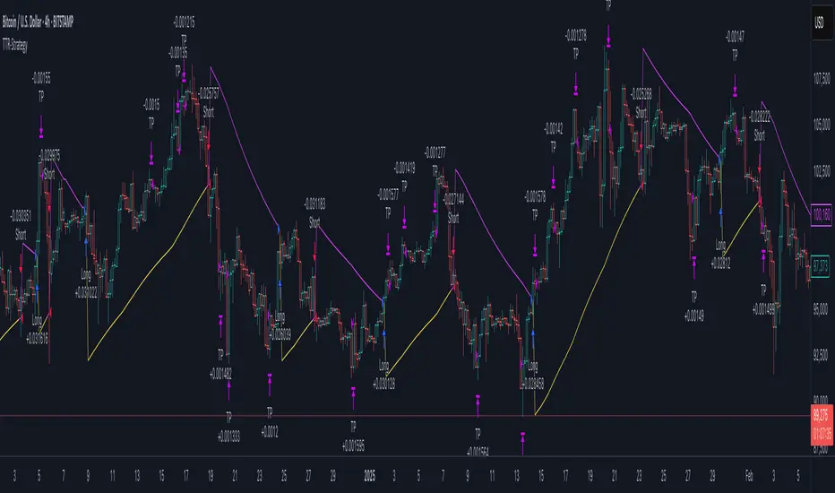
Trend Trader-Remastered StrategyOfficial Strategy for Trend Trader - Remastered
Indicator: Trend Trader-Remastered (TTR)
Overview:
The Trend Trader-Remastered is a refined and highly sophisticated implementation of the Parabolic SAR designed to create strategic buy and sell entry signals, alongside precision take profit and re-entry signals based on marked Bill Williams (BW) fractals. Built with a deep emphasis on clarity and accuracy, this indicator ensures that only relevant and meaningful signals are generated, eliminating any unnecessary entries or exits.
Please check the indicator details and updates via the link above.
Important Disclosure:
My primary objective is to provide realistic strategies and a code base for the TradingView Community. Therefore, the default settings of the strategy version of the indicator have been set to reflect realistic world trading scenarios and best practices.
Key Features:
Strategy execution date&time range.
Take Profit Reduction Rate: The percentage of progressive reduction on active position size for take profit signals.
Example:
TP Reduce: 10%
Entry Position Size: 100
TP1: 100 - 10 = 90
TP2: 90 - 9 = 81
Re-Entry When Rate: The percentage of position size on initial entry of the signal to determine re-entry.
Example:
RE When: 50%
Entry Position Size: 100
Re-Entry Condition: Active Position Size < 50
Re-Entry Fill Rate: The percentage of position size on initial entry of the signal to be completed.
Example:
RE Fill: 75%
Entry Position Size: 100
Active Position Size: 50
Re-Entry Order Size: 25
Final Active Position Size:75
Important: Even RE When condition is met, the active position size required to drop below RE Fill rate to trigger re-entry order.
Key Points:
'Process Orders on Close' is enabled as Take Profit and Re-Entry signals must be executed on candle close.
'Calculate on Every Tick' is enabled as entry signals are required to be executed within candle time.
'Initial Capital' has been set to 10,000 USD.
'Default Quantity Type' has been set to 'Percent of Equity'.
'Default Quantity' has been set to 10% as the best practice of investing 10% of the assets.
'Currency' has been set to USD.
'Commission Type' has been set to 'Commission Percent'
'Commission Value' has been set to 0.05% to reflect the most realistic results with a common taker fee value.
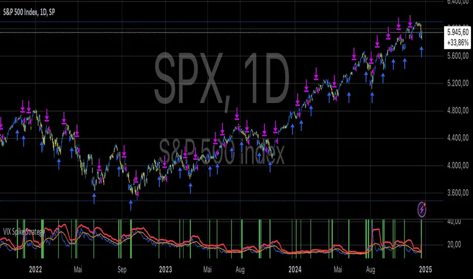
VIX Spike StrategyThis script implements a trading strategy based on the Volatility Index (VIX) and its standard deviation. It aims to enter a long position when the VIX exceeds a certain number of standard deviations above its moving average, which is a signal of a volatility spike. The position is then exited after a set number of periods.
VIX Symbol (vix_symbol): The input allows the user to specify the symbol for the VIX index (typically "CBOE:VIX").
Standard Deviation Length (stddev_length): The number of periods used to calculate the standard deviation of the VIX. This can be adjusted by the user.
Standard Deviation Multiplier (stddev_multiple): This multiplier is used to determine how many standard deviations above the moving average the VIX must exceed to trigger a long entry.
Exit Periods (exit_periods): The user specifies how many periods after entering the position the strategy will exit the trade.
Strategy Logic:
Data Loading: The script loads the VIX data, both for the current timeframe and as a rescaled version for calculation purposes.
Standard Deviation Calculation: It calculates both the moving average (SMA) and the standard deviation of the VIX over the specified period (stddev_length).
Entry Condition: A long position is entered when the VIX exceeds the moving average by a specified multiple of its standard deviation (calculated as vix_mean + stddev_multiple * vix_stddev).
Exit Condition: After the position is entered, it will be closed after the user-defined number of periods (exit_periods).
Visualization:
The VIX is plotted in blue.
The moving average of the VIX is plotted in orange.
The threshold for the VIX, which is the moving average plus the standard deviation multiplier, is plotted in red.
The background turns green when the entry condition is met, providing a visual cue.
Sources:
The VIX is often used as a measure of market volatility, with high values indicating increased uncertainty in the market.
Standard deviation is a statistical measure of the variability or dispersion of a set of data points. In financial markets, it is used to measure the volatility of asset prices.
References:
Bollerslev, T. (1986). "Generalized Autoregressive Conditional Heteroskedasticity." Journal of Econometrics.
Black, F., & Scholes, M. (1973). "The Pricing of Options and Corporate Liabilities." Journal of Political Economy.
DAILY Supertrend + EMA Crossover with RSI FilterThis strategy is a technical trading approach that combines multiple indicators—Supertrend, Exponential Moving Averages (EMAs), and the Relative Strength Index (RSI)—to identify and manage trades.
Core Components:
1. Exponential Moving Averages (EMAs):
Two EMAs, one with a shorter period (fast) and one with a longer period (slow), are calculated. The idea is to spot when the faster EMA crosses above or below the slower EMA. A fast EMA crossing above the slow EMA often suggests upward momentum, while crossing below suggests downward momentum.
2. Supertrend Indicator:
The Supertrend uses Average True Range (ATR) to establish dynamic support and resistance lines. These lines shift above or below price depending on the prevailing trend. When price is above the Supertrend line, the trend is considered bullish; when below, it’s considered bearish. This helps ensure that the strategy trades only in the direction of the overall trend rather than against it.
3. RSI Filter:
The RSI measures momentum. It helps avoid buying into markets that are already overbought or selling into markets that are oversold. For example, when going long (buying), the strategy only proceeds if the RSI is not too high, and when going short (selling), it only proceeds if the RSI is not too low. This filter is meant to improve the quality of the trades by reducing the chance of entering right before a reversal.
4. Time Filters:
The strategy only triggers entries during user-specified date and time ranges. This is useful if one wants to limit trading activity to certain trading sessions or periods with higher market liquidity.
5. Risk Management via ATR-based Stops and Targets:
Both stop loss and take profit levels are set as multiples of the ATR. ATR measures volatility, so when volatility is higher, both stops and profit targets adjust to give the trade more breathing room. Conversely, when volatility is low, stops and targets tighten. This dynamic approach helps maintain consistent risk management regardless of market conditions.
Overall Logic Flow:
- First, the market conditions are analyzed through EMAs, Supertrend, and RSI.
- When a buy (long) condition is met—meaning the fast EMA crosses above the slow EMA, the trend is bullish according to Supertrend, and RSI is below the specified “overbought” threshold—the strategy initiates or adds to a long position.
- Similarly, when a sell (short) condition is met—meaning the fast EMA crosses below the slow EMA, the trend is bearish, and RSI is above the specified “oversold” threshold—it initiates or adds to a short position.
- Each position is protected by an automatically calculated stop loss and a take profit level based on ATR multiples.
Intended Result:
By blending trend detection, momentum filtering, and volatility-adjusted risk management, the strategy aims to capture moves in the primary trend direction while avoiding entries at excessively stretched prices. Allowing multiple entries can potentially amplify gains in strong trends but also increases exposure, which traders should consider in their risk management approach.
In essence, this strategy tries to ride established trends as indicated by the Supertrend and EMAs, filter out poor-quality entries using RSI, and dynamically manage trade risk through ATR-based stops and targets.

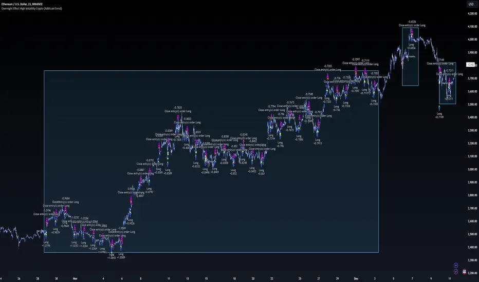
Overnight Effect High Volatility Crypto (AiBitcoinTrend)👽 Overview of the Strategy
This strategy leverages the overnight effect in the cryptocurrency market, specifically targeting the two-hour window from 21:00 UTC to 23:00 UTC. The strategy is designed to be applied only during periods of high volatility, which is determined using historical volatility data. This approach, inspired by research from Padyšák and Vojtko (2022), aims to capitalize on statistically significant return patterns observed during these hours.
Deep Backtesting with a High Volatility Filter
Deep Backtesting without a High Volatility Filter
👽 How the Strategy Works
Volatility Calculation:
Each day at 00:00 UTC, the strategy calculates the 30-day historical volatility of crypto returns (typically Bitcoin). The historical volatility is the standard deviation of the log returns over the past 30 days, representing the market's recent volatility level.
Median Volatility Benchmark:
The median of the 30-day historical volatility is calculated over a 365-day period (one year). This median acts as a benchmark to classify each day as either:
👾 High Volatility: When the current 30-day volatility exceeds the median volatility.
👾 Low Volatility: When the current 30-day volatility is below the median.
Trading Rule:
If the day is classified as a High Volatility Day, the strategy executes the following trades:
👾 Buy at 21:00 UTC.
👾 Sell at 23:00 UTC.
Trade Execution Details:
The strategy uses a 0.02% fee per trade.
Each trade is executed with 25% of the available capital. This allocation helps manage risk while allowing for compounding returns.
Rationale:
The returns during the 22:00 and 23:00 UTC hours have been found to be statistically significant during high volatility periods. The overnight effect is believed to drive this phenomenon due to the asynchronous closing hours of global financial markets. This creates unique trading opportunities in the cryptocurrency market, where exchanges remain open 24/7.
👽 Market Context and Global Time Zone Impact
👾 Why 21:00 to 23:00 UTC?
During this window, major traditional financial markets are closed:
NYSE (New York) closes at 21:00 UTC.
London and European markets are closed during these hours.
Asian markets (Tokyo, Hong Kong, etc.) open later, leaving this window largely unaffected by traditional trading flows.
This global market inactivity creates a period where significant moves can occur in the cryptocurrency market, particularly during high volatility.
👽 Strategy Parameters
Volatility Period: 30 days.
The lookback period for calculating historical volatility.
Median Period: 365 days.
The lookback period for calculating the median volatility benchmark.
Entry Time: 21:00 UTC.
Adjust this to your local time if necessary (e.g., 16:00 in New York, 22:00 in Stockholm).
Exit Time: 23:00 UTC.
Adjust this to your local time if necessary (e.g., 18:00 in New York, 00:00 midnight in Stockholm).
👽 Benefits of the Strategy
Seasonality Effect:
The strategy captures consistent patterns driven by the overnight effect and high volatility periods.
Risk Reduction:
Since trades are executed during a specific window and only on high volatility days, the strategy helps mitigate exposure to broader market risk.
Simplicity and Efficiency:
The strategy is moderately complex, making it accessible for traders while offering significant returns.
Global Applicability:
Suitable for traders worldwide, with clear guidelines on adjusting for local time zones.
👽 Considerations
Market Conditions: The strategy works best in a high-volatility environment.
Execution: Requires precise timing to enter and exit trades at the specified hours.
Time Zone Adjustments: Ensure you convert UTC times accurately based on your location to execute trades at the correct local times.
Disclaimer: This information is for entertainment purposes only and does not constitute financial advice. Please consult with a qualified financial advisor before making any investment decisions.
DCA Strategy with Mean Reversion and Bollinger BandDCA Strategy with Mean Reversion and Bollinger Band
The Dollar-Cost Averaging (DCA) Strategy with Mean Reversion and Bollinger Bands is a sophisticated trading strategy that combines the principles of DCA, mean reversion, and technical analysis using Bollinger Bands. This strategy aims to capitalize on market corrections by systematically entering positions during periods of price pullbacks and reversion to the mean.
Key Concepts and Principles
1. Dollar-Cost Averaging (DCA)
DCA is an investment strategy that involves regularly purchasing a fixed dollar amount of an asset, regardless of its price. The idea behind DCA is that by spreading out investments over time, the impact of market volatility is reduced, and investors can avoid making large investments at inopportune times. The strategy reduces the risk of buying all at once during a market high and can smooth out the cost of purchasing assets over time.
In the context of this strategy, the Investment Amount (USD) is set by the user and represents the amount of capital to be invested in each buy order. The strategy executes buy orders whenever the price crosses below the lower Bollinger Band, which suggests a potential market correction or pullback. This is an effective way to average the entry price and avoid the emotional pitfalls of trying to time the market perfectly.
2. Mean Reversion
Mean reversion is a concept that suggests prices will tend to return to their historical average or mean over time. In this strategy, mean reversion is implemented using the Bollinger Bands, which are based on a moving average and standard deviation. The lower band is considered a potential buy signal when the price crosses below it, indicating that the asset has become oversold or underpriced relative to its historical average. This triggers the DCA buy order.
Mean reversion strategies are popular because they exploit the natural tendency of prices to revert to their mean after experiencing extreme deviations, such as during market corrections or panic selling.
3. Bollinger Bands
Bollinger Bands are a technical analysis tool that consists of three lines:
Middle Band: The moving average, usually a 200-period Exponential Moving Average (EMA) in this strategy. This serves as the "mean" or baseline.
Upper Band: The middle band plus a certain number of standard deviations (multiplier). The upper band is used to identify overbought conditions.
Lower Band: The middle band minus a certain number of standard deviations (multiplier). The lower band is used to identify oversold conditions.
In this strategy, the Bollinger Bands are used to identify potential entry points for DCA trades. When the price crosses below the lower band, this is seen as a potential opportunity for mean reversion, suggesting that the asset may be oversold and could reverse back toward the middle band (the EMA). Conversely, when the price crosses above the upper band, it indicates overbought conditions and signals potential market exhaustion.
4. Time-Based Entry and Exit
The strategy has specific entry and exit points defined by time parameters:
Open Date: The date when the strategy begins opening positions.
Close Date: The date when all positions are closed.
This time-bound approach ensures that the strategy is active only during a specified window, which can be useful for testing specific market conditions or focusing on a particular time frame.
5. Position Sizing
Position sizing is determined by the Investment Amount (USD), which is the fixed amount to be invested in each buy order. The quantity of the asset to be purchased is calculated by dividing the investment amount by the current price of the asset (investment_amount / close). This ensures that the amount invested remains constant despite fluctuations in the asset's price.
6. Closing All Positions
The strategy includes an exit rule that closes all positions once the specified close date is reached. This allows for controlled exits and limits the exposure to market fluctuations beyond the strategy's timeframe.
7. Background Color Based on Price Relative to Bollinger Bands
The script uses the background color of the chart to provide visual feedback about the price's relationship with the Bollinger Bands:
Red background indicates the price is above the upper band, signaling overbought conditions.
Green background indicates the price is below the lower band, signaling oversold conditions.
This provides an easy-to-interpret visual cue for traders to assess the current market environment.
Postscript: Configuring Initial Capital for Backtesting
To ensure the backtest results align with the actual investment scenario, users must adjust the Initial Capital in the TradingView strategy properties. This is done by calculating the Initial Capital as the product of the Total Closed Trades and the Investment Amount (USD). For instance:
If the user is investing 100 USD per trade and has 10 closed trades, the Initial Capital should be set to 1,000 USD.
Similarly, if the user is investing 200 USD per trade and has 24 closed trades, the Initial Capital should be set to 4,800 USD.
This adjustment ensures that the backtesting results reflect the actual capital deployed in the strategy and provides an accurate representation of potential gains and losses.
Conclusion
The DCA strategy with Mean Reversion and Bollinger Bands is a systematic approach to investing that leverages the power of regular investments and technical analysis to reduce market timing risks. By combining DCA with the insights offered by Bollinger Bands and mean reversion, this strategy offers a structured way to navigate volatile markets while targeting favorable entry points. The clear entry and exit rules, coupled with time-based constraints, make it a robust and disciplined approach to long-term investing.

Precision Trading Strategy: Golden EdgeThe PTS: Golden Edge strategy is designed for scalping Gold (XAU/USD) on lower timeframes, such as the 1-minute chart. It captures high-probability trade setups by aligning with strong trends and momentum, while filtering out low-quality trades during consolidation or low-volatility periods.
The strategy uses a combination of technical indicators to identify optimal entry points:
1. Exponential Moving Averages (EMAs): A fast EMA (3-period) and a slow EMA (33-period) are used to detect short-term trend reversals via crossover signals.
2. Hull Moving Average (HMA): A 66-period HMA acts as a higher-timeframe trend filter to ensure trades align with the overall market direction.
3. Relative Strength Index (RSI): A 12-period RSI identifies momentum. The strategy requires RSI > 55 for long trades and RSI < 45 for short trades, ensuring entries are backed by strong buying or selling pressure.
4. Average True Range (ATR): A 14-period ATR ensures trades occur only during volatile conditions, avoiding choppy or low-movement markets.
By combining these tools, the PTS: Golden Edge strategy creates a precise framework for scalping and offers a systematic approach to capitalize on Gold’s price movements efficiently.

BTCUSD Momentum After Abnormal DaysThis indicator identifies abnormal days in the Bitcoin market (BTCUSD) based on daily returns exceeding specific thresholds defined by a statistical approach. It is inspired by the findings of Caporale and Plastun (2020), who analyzed the cryptocurrency market's inefficiencies and identified exploitable patterns, particularly around abnormal returns.
Key Concept:
Abnormal Days:
Days where the daily return significantly deviates (positively or negatively) from the historical average.
Positive abnormal days: Returns exceed the mean return plus k times the standard deviation.
Negative abnormal days: Returns fall below the mean return minus k times the standard deviation.
Momentum Effect:
As described in the academic paper, on abnormal days, prices tend to move in the direction of the abnormal return until the end of the trading day, creating momentum effects. This can be leveraged by traders for profit opportunities.
How It Works:
Calculation:
The script calculates the daily return as the percentage difference between the open and close prices. It then derives the mean and standard deviation of returns over a configurable lookback period.
Thresholds:
The script dynamically computes upper and lower thresholds for abnormal days using the mean and standard deviation. Days exceeding these thresholds are flagged as abnormal.
Visualization:
The mean return and thresholds are plotted as dynamic lines.
Abnormal days are visually highlighted with transparent green (positive) or red (negative) backgrounds on the chart.
References:
This indicator is based on the methodology discussed in "Momentum Effects in the Cryptocurrency Market After One-Day Abnormal Returns" by Caporale and Plastun (2020). Their research demonstrates that hourly returns during abnormal days exhibit a strong momentum effect, moving in the same direction as the abnormal return. This behavior contradicts the efficient market hypothesis and suggests profitable trading opportunities.
"Prices tend to move in the direction of abnormal returns till the end of the day, which implies the existence of a momentum effect on that day giving rise to exploitable profit opportunities" (Caporale & Plastun, 2020).

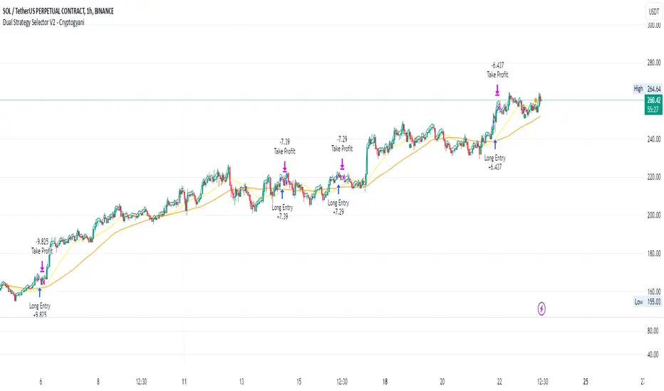
Dual Strategy Selector V2 - CryptogyaniOverview:
This script provides traders with a dual-strategy system that they can toggle between using a simple dropdown menu in the input settings. It is designed to cater to different trading styles and needs, offering both simplicity and advanced filtering techniques. The strategies are built around moving average crossovers, enhanced by configurable risk management tools like take profit levels, trailing stops, and ATR-based stop-loss.
Key Features:
Two Strategies in One Script:
Strategy 1: A classic moving average crossover strategy for identifying entry signals based on trend reversals. Includes user-defined take profit and trailing stop-loss options for profit locking.
Strategy 2: An advanced trend-following system that incorporates:
A higher timeframe trend filter to confirm entry signals.
ATR-based stop-loss for dynamic risk management.
Configurable partial take profit to secure gains while letting the trade run.
Highly Customizable:
All key parameters such as SMA lengths, take profit levels, ATR multiplier, and timeframe for the trend filter are adjustable via the input settings.
Dynamic Toggle:
Traders can switch between Strategy 1 and Strategy 2 with a single dropdown, allowing them to adapt the strategy to market conditions.
How It Works:
Strategy 1:
Entry Logic: A long trade is triggered when the fast SMA crosses above the slow SMA.
Exit Logic: The trade exits at either a user-defined take profit level (percentage or pips) or via an optional trailing stop that dynamically adjusts based on price movement.
Strategy 2:
Entry Logic: Builds on the SMA crossover logic but adds a higher timeframe trend filter to align trades with the broader market direction.
Risk Management:
ATR-Based Stop-Loss: Protects against adverse moves with a volatility-adjusted stop-loss.
Partial Take Profit: Allows traders to secure a percentage of gains while keeping some exposure for extended trends.
How to Use:
Select Your Strategy:
Use the dropdown in the input settings to choose Strategy 1 or Strategy 2.
Configure Parameters:
Adjust SMA lengths, take profit, and risk management settings to align with your trading style.
For Strategy 2, specify the higher timeframe for trend filtering.
Deploy and Monitor:
Apply the script to your preferred asset and timeframe.
Use the backtest results to fine-tune settings for optimal performance.
Why Choose This Script?:
This script stands out due to its dual-strategy flexibility and enhanced features:
For beginners: Strategy 1 provides a simple yet effective trend-following system with minimal setup.
For advanced traders: Strategy 2 includes powerful tools like trend filters and ATR-based stop-loss, making it ideal for challenging market conditions.
By combining simplicity with advanced features, this script offers something for everyone while maintaining full transparency and user customization.
Default Settings:
Strategy 1:
Fast SMA: 21, Slow SMA: 49
Take Profit: 7% or 50 pips
Trailing Stop: Optional (disabled by default)
Strategy 2:
Fast SMA: 20, Slow SMA: 50
ATR Multiplier: 1.5
Partial Take Profit: 50%
Higher Timeframe: 1 Day (1D)
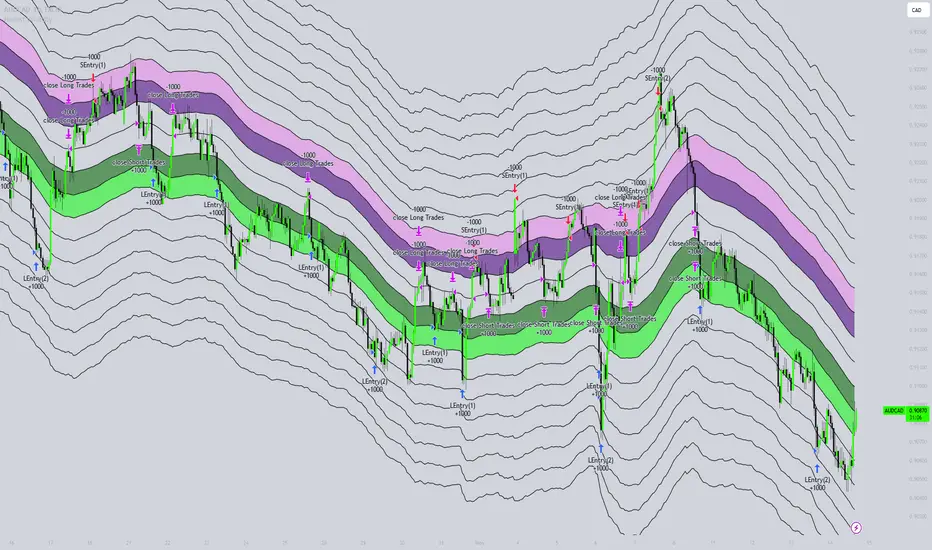
Honest Volatility Grid [Honestcowboy]The Honest Volatility Grid is an attempt at creating a robust grid trading strategy but without standard levels.
Normal grid systems use price levels like 1.01;1.02;1.03;1.04... and place an order at each of these levels. In this program instead we create a grid using keltner channels using a long term moving average.
🟦 IS THIS EVEN USEFUL?
The idea is to have a more fluid style of trading where levels expand and follow price and do not stick to precreated levels. This however also makes each closed trade different instead of using fixed take profit levels. In this strategy a take profit level can even be a loss. It is useful as a strategy because it works in a different way than most strategies, making it a good tool to diversify a portfolio of trading strategies.
🟦 STRATEGY
There are 10 levels below the moving average and 10 above the moving average. For each side of the moving average the strategy uses 1 to 3 orders maximum (3 shorts at top, 3 longs at bottom). For instance you buy at level 2 below moving average and you increase position size when level 6 is reached (a cheaper price) in order to spread risks.
By default the strategy exits all trades when the moving average is reached, this makes it a mean reversion strategy. It is specifically designed for the forex market as these in my experience exhibit a lot of ranging behaviour on all the timeframes below daily.
There is also a stop loss at the outer band by default, in case price moves too far from the mean.
What are the risks?
In case price decides to stay below the moving average and never reaches the outer band one trade can create a very substantial loss, as the bands will keep following price and are not at a fixed level.
Explanation of default parameters
By default the strategy uses a starting capital of 25000$, this is realistic for retail traders.
Lot sizes at each level are set to minimum lot size 0.01, there is no reason for the default to be risky, if you want to risk more or increase equity curve increase the number at your own risk.
Slippage set to 20 points: that's a normal 2 pip slippage you will find on brokers.
Fill limit assumtion 20 points: so it takes 2 pips to confirm a fill, normal forex spread.
Commission is set to 0.00005 per contract: this means that for each contract traded there is a 5$ or whatever base currency pair has as commission. The number is set to 0.00005 because pinescript does not know that 1 contract is 100000 units. So we divide the number by 100000 to get a realistic commission.
The script will also multiply lot size by 100000 because pinescript does not know that lots are 100000 units in forex.
Extra safety limit
Normally the script uses strategy.exit() to exit trades at TP or SL. But because these are created 1 bar after a limit or stop order is filled in pinescript. There are strategy.orders set at the outer boundaries of the script to hedge against that risk. These get deleted bar after the first order is filled. Purely to counteract news bars or huge spikes in price messing up backtest.
🟦 VISUAL GOODIES
I've added a market profile feature to the edge of the grid. This so you can see in which grid zone market has been the most over X bars in the past. Some traders may wish to only turn on the strategy whenever the market profile displays specific characteristics (ranging market for instance).
These simply count how many times a high, low, or close price has been in each zone for X bars in the past. it's these purple boxes at the right side of the chart.
🟦 Script can be fully automated to MT5
There are risk settings in lot sizes or % for alerts and symbol settings provided at the bottom of the indicator. The script will send alert to MT5 broker trying to mimic the execution that happens on tradingview. There are always delays when using a bridge to MT5 broker and there could be errors so be mindful of that. This script sends alerts in format so they can be read by tradingview.to which is a bridge between the platforms.
Use the all alert function calls feature when setting up alerts and make sure you provide the right webhook if you want to use this approach.
Almost every setting in this indicator has a tooltip added to it. So if any setting is not clear hover over the (?) icon on the right of the setting.
BarRange StrategyHello,
This is a long-only, volatility-based strategy that analyzes the range of the previous bar (high - low).
If the most recent bar’s range exceeds a threshold based on the last X bars, a trade is initiated.
You can customize the lookback period, threshold value, and exit type.
For exits, you can choose to exit after X bars or when the close price exceeds the previous bar’s high.
The strategy is designed for instruments with a long-term upward-sloping curves, such as ES1! or NQ1!. It may not perform well on other instruments.
Commissions are set to $2.50 per side ($5.00 per round trip).
Recommended timeframes are 1h and higher. With adjustments to the lookback period and threshold, it could potentially achieve similar results on lower timeframes as well.

Zig Zag + Aroon StrategyBelow is a trading strategy that combines the Zig Zag indicator and the Aroon indicator. This combination can help identify trends and potential reversal points.
Zig Zag and Aroon Strategy Overview
Zig Zag Indicator:
The Zig Zag indicator helps to identify significant price movements and eliminates smaller fluctuations. It is useful for spotting trends and reversals.
Aroon Indicator:
The Aroon indicator consists of two lines: Aroon Up and Aroon Down. It measures the time since the highest high and the lowest low over a specified period, indicating the strength of a trend.
Strategy Conditions
Long Entry Conditions:
Aroon Up crosses above Aroon Down (indicating a bullish trend).
The Zig Zag indicator shows an upward movement (indicating a potential continuation).
Short Entry Conditions:
Aroon Down crosses above Aroon Up (indicating a bearish trend).
The Zig Zag indicator shows a downward movement (indicating a potential continuation).
Exit Conditions:
Exit long when Aroon Down crosses above Aroon Up.
Exit short when Aroon Up crosses above Aroon Down.
